
A DolphinDB-Based Study of Price Wicking in Cryptocurrency Markets
Since the inception of Bitcoin, cryptocurrency markets have been known for their high volatility. Flash crashes and price wicks (also referred to as "needle-like bars") are typical extreme price patterns that frequently appear in OHLC bar charts across major exchanges. A flash crash refers to an extreme market event in which the price of a crypto asset plunges dramatically within a very short period, with a large decline and a sudden evaporation of liquidity. A price wick, by contrast, is a distinctive price pattern in which the price briefly breaks through a key support or resistance level by a large margin, leaves a long upper or lower shadow on the OHLC bar chart, and then quickly returns to its original range. These extreme events not only cause highly leveraged traders to be liquidated instantly, but also intensify market panic and may trigger cascading liquidations, creating systemic risk across the broader market. Therefore, it is both theoretically valuable and practically important to identify extreme price patterns such as price wicks in a rigorous way, uncover their micro-level formation mechanisms, and build effective risk warning and prevention mechanisms. Using DolphinDB, this article focuses on the following topics:
- The background and definition of price wicking
- The relationship between price wicking and high-frequency indicators such as order flow toxicity (VPIN) and order book imbalance
- An analysis, based on real data, of changes in liquidation data, order book depth, and trading volume during a typical event (the event on October 10, 2025)
- A risk control and early warning approach based on the VPIN indicator
1. Background and Definition of Price Wicking
Compared with traditional markets, cryptocurrency markets are more prone to sharp price swings and rapid up-and-down movements, known as price wicking, due to their 24/7 trading nature, fragmented liquidity, and diverse liquidation mechanisms. To support a better understanding and analysis of this extreme market behavior, this chapter introduces the theoretical background of price wicking and methods for defining them quantitatively.
1.1 Theoretical Background
From theoretical and market microstructure perspectives, price wicking is mainly driven by the following factors:
- Informed Trading: Large institutions or traders with private information buy or sell an asset in large quantities over a given period, causing sharp short-term price fluctuations.
- Insufficient Market Liquidity: Especially in markets with low trading volume, such as certain small cryptocurrency pairs, large orders entering or exiting the market can cause prices to move sharply in an instant.
- Market Manipulation: Some market participants may deliberately influence prices through large-scale buying or selling, thereby triggering price wicking.
- Leverage and Forced Liquidation Mechanisms: High leverage in perpetual futures contracts, combined with forced liquidation rules, means that even a small price deviation can trigger cascading liquidations. Liquidation orders then amplify the market move, creating a "price wicking-liquidation-price wicking" feedback loop.
In addition, an exchange's liquidation mechanism directly affects the magnitude of market impact:
- Full Forced Liquidation: Once triggered, the entire position is immediately liquidated at market price. This mechanism is simple but blunt. When a large position is liquidated, it can drain liquidity instantly and is highly likely to trigger a chain of further liquidations.
- Partial Forced Liquidation: Exchanges such as Binance use this mechanism. The system first attempts to close part of the position so that the margin ratio returns above the maintenance threshold, which in theory reduces market impact. However, during the extreme market conditions of October 2025, prices fell so rapidly that the partial forced liquidation mechanism failed. The system was forced to trigger forced liquidations repeatedly, producing an effect equivalent to full forced liquidation [1].
1.2 Quantitative Definition
In trading contexts, a "price wick" is essentially a type of extreme OHLC bar pattern: it has a long shadow, a small body, and a price range significantly larger than normal. In terms of its origins, the qualitative description of this type of pattern in classic candlestick analysis can be traced back to Steve Nison's systematic study of candlestick charting techniques [2]. Traditional definitions, however, are mostly qualitative. To quantify the definition of a "price wick" intuitively, this article uses a pattern-ratio method and represents a price wick as follows:
- The shadow length is significantly larger than the body length;
- The shadow length accounts for a large proportion of the total OHLC bar range;
- The total OHLC bar range reaches a specified absolute or relative threshold, filtering out ordinary bid-ask spread fluctuations.
The shadow, body, and range are defined as follows:
- Upper shadow length:
upper = high - max(open,close) - Lower shadow length:
lower = min(open,close) - low - Body length:
body = |open -close| - Range:
amplitude = high - low
The specific formula is as follows:
2. Core Monitoring Indicators
Investigating the causes and patterns of price wicking requires an in-depth analysis of market microstructure data. This chapter introduces two core high-frequency monitoring indicators: VPIN-based order flow toxicity and order book imbalance. Both are applied directly in the case study in Chapter 3.
2.1 VPIN: A Measure of Order Flow Toxicity
VPIN (Volume-Synchronized Probability of Informed Trading) is a high-frequency indicator for measuring order flow toxicity, proposed by Easley et al. in 2011 [3]. It measures the degree of information asymmetry in order flow, or "toxicity". The core idea is to "measure time by trading volume": time is divided into volume buckets with equal trading volume, and order imbalance is measured by calculating the difference between aggressive buy and sell orders in each bucket.
The formula is as follows:
Here, V is the fixed trading volume of each bucket, and
n is the number of buckets in the calculation window. The
numerator is the absolute value of the difference between aggressive buy and
sell trading volume, representing order flow imbalance.
Before calculating VPIN, you need to determine the number of buckets and the
fixed trading volume per bucket. In this article, the bucket volume
V is set to the average daily trading volume over the past 20
trading days divided by N, with N set to 50
buckets per day.
Next, calculate and sum the imbalance between aggressive buy and sell orders in
each bucket. Finally, normalize the result by dividing it by the number of
buckets n in the calculation window and the fixed trading
volume V.
2. Total trading volume is equal to the sum of aggressive buy trading volume and aggressive sell trading volume within the bucket.
2.2 Order Book Imbalance
From the perspective of basic indicators, price wicking is often accompanied by changes in the order book depth ratio and the funding rate:
- Order Book Depth Ratio: The ratio of cumulative resting order volume
from the best bid to the Nth bid level to cumulative resting order volume
from the best ask to the Nth ask level. When this ratio drops sharply, it
indicates that downside support has weakened and that there is less
resistance to a price decline [4].
Therefore, two related indicators can be constructed:
Depth Ratio
Normalized Imbalance
Here,
bidDepthandaskDepthrepresent the cumulative order quantity (or notional amount) from bid/ask level 1 through bid/ask level N, respectively. - Funding Rate: The degree to which the perpetual futures contract price deviates from the spot price. An extremely negative funding rate indicates that the market is highly bearish, but it may also signal a reversal wick caused by a short squeeze. An extremely positive funding rate suggests overcrowded long positions, which can easily trigger a long liquidation cascade.
3. Case Study
Building on the theoretical analysis in Chapters 1 and 2, this chapter uses the DolphinDB scripts and real market data to further analyze price wicking in cryptocurrency markets. Note that all related data has been stored in a DolphinDB DFS database. If your database and table schemas or field names differ, modify the sample scripts accordingly. To run a simulation, you can obtain the data files from the attachment and update the data-loading section in the sample scripts. For the specific data solution used, see DolphinDB-Based Solution for Quantitative Cryptocurrency Trading.
3.1 Price Wicking Definition
Based on minute-level OHLC bar data and the criteria described in Chapter 1, the relevant code is as follows:
symList = ["BTCUSDT"]
sySource =  "Binance-Futures"
dataKline = select * from loadTable("dfs://CryptocurrencyKLine","minKLine") where
      symbol in symList and symbolSource = sySource  order by eventTime
//If the data uses UTC + 8h, standardize it to UTC time:
// update dataKline set eventTime = temporalAdd(eventTime, -8, 'h')
//Downsample the data:
//barMinutes = 5
//dataKline = select eventTime, sym, sySource, first(open) as open,
//	max(high) as high, min(low) as low, last(close) as close, sum(volume) as volume
//    from dataKline group by bar(eventTime, barMinutes*60*1000) as eventTime
//The shadow is significantly longer than the real body
update dataKline set body = abs(close - open)
update dataKline set amplitude  = (high - low)
update dataKline set upper = (high - max(open,close))
update dataKline set lower = (min(open,close) - low)
update dataKline set avgPrice = (open + close)/2
//Detection criteria; modify as needed
a,b,c = 5.0,0.5,0.5
pinbar = select * from dataKline where lower > body * a and lower > amplitude * b
pinbar_upper = select * from dataKline where upper > body * a and upper > amplitude * b
pinbar.append!(pinbar_upper)
pinbar = select * from pinbar where amplitude > avgPrice*c*0.01 order by eventTime
Line 6 standardizes the time zone to UTC. Lines 20 and 21 define the core
criteria for detecting price wicking. To use the upper shadow instead, use
upper. If you need to downsample OHLC bars at different
frequencies, modify barMinutes accordingly.
Using 5-minute OHLC bar data for BTCUSDT on Binance as an example, the sample results are as follows:

The results show that OHLC bars matching price wicking are often accompanied by large trading volume, especially compared with the average trading volume for the day. For example, at 2025.10.10T21:20:00.000 in the figure, the low price reached 101,516.5, about 7,000 below the opening price of 108,888, before rebounding to a closing price of 107,747.3. The trading volume in this interval was roughly an order of magnitude higher than in other periods.
3.2 VPIN Calculation
The VPIN-related functions and volatility analytic functions are encapsulated in
the CalcVPINModule module. For the complete code, see the attached file
CalcVPINModule.dos. The module contains the following
functions:
| Function Name | Description | Note |
|---|---|---|
calcBucketSize |
Function for calculating bucket size V | By default, V is calculated as the average daily trading volume over the previous 20 days divided by 50 buckets per day. |
bucketizeForTrade |
Function for bucketizing trade data | For the data structure, see Section 2.1, Database and Table Schemas, in DolphinDB-Based Solution for Quantitative Cryptocurrency Trading. |
bucketizeForKline |
Function for bucketizing minKLine data | Same as above |
calcVPINForAllSym |
Function for calculating VPIN | Concurrent calculation for multiple currencies on a single trading day |
calcVPINVolCor |
Function for calculating volatility and correlation | Includes price range volatility, log returns, Parkinson volatility, and more. You can modify or extend it as needed. |
Usage:
- Place the module file in the
<path returned by
                            getHomeDir()>/modules
path, and then call it withuse:use CalcVPINModule - Set the parameters as needed, and choose either parallel or serial execution
to calculate VPIN values across multiple days:
symList = [`BTCUSDT,`ETHUSDT,`XRPUSDT,`ADAUSDT] targetSource = "Binance-Futures" // Or "OKX-Futures" dataType = "trade" //"trade" or "minKLine" d,N,n = 20,50,10 //Use the previous d days and N buckets per day to calculate V, with a window size of n //Run parallel calculations across multiple trading days: Date = 2025.10.01..2025.10.30 //UTC time result = peach(calcVPINForAllSym{,symList,targetSource,dataType,d, N,n}, Date) res = select * from unionAll(result) order by symbol, eventTime //If memory is limited, run the calculation serially res = table(1000:0, `eventTime`symbolSource`symbol`diffQty`VPIN`price_open`price_high`price_low `price_close`price_range`bucket_volume, [TIMESTAMP, SYMBOL, SYMBOL, DOUBLE, DOUBLE, DOUBLE, DOUBLE, DOUBLE, DOUBLE, DOUBLE, DOUBLE]) for(targetDate in Date){ res_VPIN = calcVPINForAllSym(targetDate,symList,targetSource,dataType,d, N,n) res.append!(res_VPIN) } resis the table containing the VPIN calculation results. You can also call thecalcVPINVolCorfunction to obtain basic volatility and correlation results:result = calcVPINVolCor(res) result- Finally, use DolphinDB's built-in plot function to draw the chart:
sym = "ADAUSDT"
plotData = select * from res where symbol = sym
plot(plotData[`volatility_range`VPIN],plotData.eventTime,sym +":VPIN vs Volatility",extras={multiYAxes: true})
plot(plotData[`volatility_log`VPIN],plotData.eventTime,sym +":|Log Return| (%)",extras={multiYAxes: true})
Sample Results:
Based on aggregated trade data, the following example shows the VPIN and volatility results for October 2025:


The sample volatility correlation results are as follows:
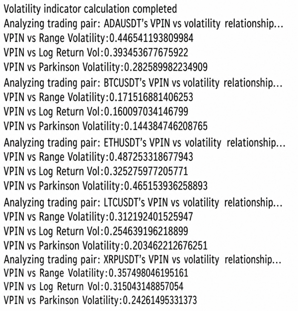
To show the relationship between VPIN and volatility more clearly, the following comparison charts are plotted:
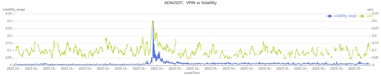


The charts show a clear synchronization between VPIN and volatility for ADAUSDT and ETHUSDT in October 2025, especially around the extreme market event on October 10, 2025. This indicates that rising order flow toxicity is typically accompanied by amplified short-term price volatility. In normal market conditions, however, the linkage between the two is relatively weak. In addition, across cryptocurrencies, BTC showed a relatively weaker relationship between VPIN and volatility during this period, possibly because its larger market capacity and stronger liquidity absorption make it more resilient. By contrast, a smaller cryptocurrency such as ADA, with weaker liquidity and insufficient order book depth, is more likely to translate order flow imbalance into significant price volatility.
3.3 Order Book Imbalance
Building on the definition of order book imbalance introduced earlier, this
section further analyzes the relationship between this metric and price wicking.
The basic calculation procedure is as follows. For the complete code, see the
attachment CalcDepthRatioModule.dos.
- Retrieve order book depth data and calculate the imbalance metric based on the definition.
- Use the last snapshot in each minute to avoid signal dilution caused by averaging multiple snapshots.
- Calculate future price returns and amplitudes over different window lengths.
- Use the quantiles of the order book imbalance metric
depthRatioQtyDifffor each symbol as thresholds to identify depth imbalance spikes. - Then compare the relationship between spikes and future amplitude by
calculating
ampRatio= future amplitude with spikes / future amplitude without spikes.
Usage:
The steps above are encapsulated into corresponding functions. To run the
analysis, call the main function depthRatioAnalysis:
use CalcDepthRatioModule
symList = [`BTCUSDT,`XRPUSDT,`ETHUSDT,`ADAUSDT]
targetSource = "Binance-Futures"
targetDate = 2025.10.10  //Supports an input time range
futureStep = 5  //Number of future amplitude windows
Data, spikeComparisonForSym, corrForSym = depthRatioAnalysis(symList,targetSource,targetDate,futureStep)
After obtaining the results, use DolphinDB's built-in plot
function to chart the data for a single symbol:
//Plot data for a single symbol
sym = "ADAUSDT"
plotData = select * from Data where symbol = sym order by timestamp
update plotData set priceChange = (highPrice - lowPrice) / highPrice
// Compare the current depth metric with the current price change
plot(plotData[`priceChange`depthRatioPrice],plotData.timestamp.minute(),
    sym + " priceChange vs depthRatioPrice", extras={multiYAxes: true})
plot(plotData[`priceChange`depthRatioPriceDiff],plotData.timestamp.minute(),
    sym + " priceChange vs depthRatioPriceDiff", extras={multiYAxes: true})

// Compare the depth metric with future returns
plot(plotData[`futureRet5`depthRatioPrice], plotData.timestamp, sym + " futureRet5 vs depthRatioPrice",
    extras={multiYAxes: true})
plot(plotData[`futureRet5`depthRatioPriceDiff], plotData.timestamp, sym + " futureRet5 vs depthRatioPriceDiff",
    extras={multiYAxes: true})
Example Results:
Using the parameters in the example above, the following table shows sample
Data output for the order book imbalance metric on October 10,
2025:

After filtering for imbalance spikes, the relationship with the future 5-minute
amplitude is shown below. Here, ampRatio is the ratio of the
future 5-minute amplitude during spike periods to the future 5-minute amplitude
during non-spike periods:

To illustrate the relationship between the order book imbalance metric and price volatility more clearly, the following comparison charts are plotted:


The relationship table for depth spikes and future amplitude shows that when
depthRatioQtyDiff experiences a sharp move at the
90th-percentile level within a single symbol, the future 5-minute amplitudes of
BTC, ETH, and XRP increase significantly, with ampRatio values
of approximately 2.20, 2.00, and 3.42, respectively. This indicates that, for
these symbols, depth spikes are indeed associated with subsequent increases in
short-term volatility and can provide a degree of early warning for price wick
events. By contrast, the ADA results are unusually unstable, indicating
potential issues with the data or threshold settings for this symbol. ADA
therefore cannot be included directly in the same conclusion.
The two depthRatioPrice and priceChange charts show no stable linear relationship in which the order book depth imbalance signal consistently precedes future price amplitude. In the later period from 21:10 to 22:50, priceChange fluctuated sharply and displayed price wick peaks, accompanied by severe fluctuations in market liquidity as measured by depthRatioPrice. In other words, this metric is suitable for risk and volatility signal detection as well as price wick identification, and can serve as an early warning signal for price wicking.
3.4 Analysis of the Event on October 10, 2025
Event Background:
On the evening of October 10, 2025, U.S. President Donald Trump announced a 100% tariff on all Chinese imports and new export controls on critical software. This unexpected geopolitical escalation immediately triggered risk-off sentiment across global markets. The S&P 500 fell 2.7%, Bitcoin plunged by more than 14%, Ethereum declined by approximately 12%, and smaller altcoins suffered even larger losses, with many dropping 40% to 70% before partially recovering [5]. Within several hours between October 10 and October 11, more than USD 19 billion in leveraged positions were liquidated, making it one of the largest single-day liquidation events in crypto history.
At the microstructure level, the crash occurred on a Friday evening in the United States, when institutional market makers were entering the weekend period and market liquidity was near a low point. Bitcoin had just reached a new all-time high of approximately USD 125,000, and the market was crowded with overleveraged long positions, creating highly fragile conditions.
Analysis Using Real Data:
- Based on the pinbar table (price wick identification result) from Section
4.1, we filter for minute-level OHLC bars on October 10, 2025 that meet the
price wicking criteria. Some examples are shown below:
pinbar_= select * from pinbar where date(eventTime)=2025.10.10 and symbol = "BTCUSDT"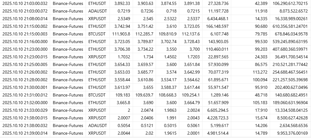
Figure 12. Figure 3-12: Price Wick Identification on October 10, 2025 As shown above, prices fluctuated significantly between 21:00 and 22:00, during which many price wicks occurred.
- Liquidation data is one of the core datasets for studying price wicking. It
reflects the precise price levels where major participants target and flush
out highly leveraged positions, the cascading effect of serial liquidations,
and the real impact of market liquidity depletion. The code example and
results are as follows:
liqDataForSym = select * from loadTable("dfs://CryptocurrencyDay","liquidation")
update liqDataForSym set eventTime = temporalAdd(eventTime, -8, "H")  //Normalize to UTC time
liqDataForSymDay = select sum(quantity),side, date,symbolSource from liqDataForSym
    group by symbolSource,side, date(eventTime) as date
res1 = select * from liqDataForSymDay order by date
liqDataForOneDay = select sum(quantity), side,eventTime,symbolSource from liqDataForSym
    where date(eventTime) = 2025.10.10 group by symbolSource,side, bar(eventTime,1m) as eventTime
res2 =select * from liqDataForOneDay order by sum_quantity desc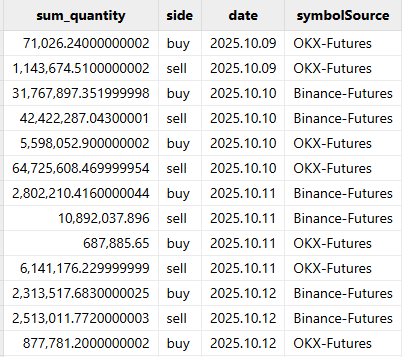
Figure 13. Figure 3-13: Daily Liquidation Data res1 Statistics 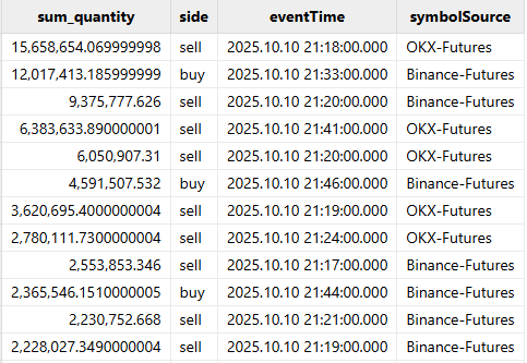
Figure 14. Figure 3-14: Intraday Minute-Level Liquidation Data res2 Statistics The charts above show liquidation data from different exchanges (OKX-Futures and Binance-Futures) for selected dates and intraday minutes. The liquidation volume on October 10, 2025 was far higher than on other dates, with a large number of leveraged traders facing forced liquidation. Sell-side liquidations greatly exceeded buy-side liquidations, highlighting the extreme volatility in market sentiment on that day. On October 10, 2025, liquidation volumes were extremely large between 21:10 and 22:00, corresponding to the severe price volatility around that period. Using XRPUSDT as an example, the relationship between minute-level liquidation data and price changes is shown below:

Figure 15. Figure 3-15: Liquidation Data and Price Changes As shown above, liquidation activity spiked between 21:00 and 22:00, coinciding with sharp price volatility and highlighting the close relationship between liquidations and price movements.
- Order book depth is an important metric for measuring market liquidity and
the market's capacity to absorb price pressure. Because the order book depth
data used here covers only a limited number of levels, we use the difference
between the best bid and best ask prices to represent market liquidity. A
wider spread typically indicates poorer liquidity and higher price
volatility risk. The code example and results are as follows:
//...
data = select * from loadTable("dfs://CryptocurrencyTick","depth")
    where symbol = "BTCUSDT" and symbolSource = sySource and eventTime between startTargetTime:endTargetTime
update data set eventTime = temporalAdd(eventTime, -8, "H") //Normalize to UTC time
plotData = select eventTime,symbolSource,symbol,(bidQty[0]-askQty[0]) as diffQty from data
// Overall difference across multiple bid and ask price levels
// plotData = select eventTime,symbolSource,symbol,each(sum,bidQty-askQty) as diffQty from data
plot(plotData[`diffQty],plotData.eventTime.minute(),"bid-ask spread",extras={multiYAxes: true})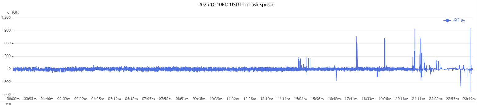
Figure 16. Figure 3-16: Bid-Ask Spread Changes As shown above, order book depth experienced several large fluctuations during the day, with the most severe movements occurring between 21:00 and 22:10. This reflected an extreme order flow imbalance, and made price wick events more likely.
- Trading volume is one of the core factors that drives price volatility and
is essential for analyzing price wick events. The data used in this section
is aggregated trade data provided by the exchange. It includes only regular
market orders and excludes special orders such as liquidation and forced
liquidation orders. The following are the single-day trading volume summary
table and the chart showing the relationship between intraday trading volume
and price for the XRPUSDT trading pair:
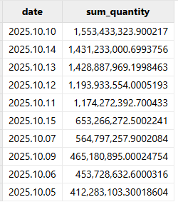
Figure 17. Figure 3-17: Single-Day Trading Volume Chart 
Figure 18. Figure 3-18: Intraday Trading Volume and Price Relationship Chart for a Single Trading Pair Based on the market trading volume for "XRPUSDT" on that day, trading volume increased sharply after 20:50, indicating a significant shift in market sentiment. A large influx of orders disrupted the supply-demand balance and directly amplified price fluctuations, demonstrating the impact of substantial trading volume on price volatility.
4. Risk Control
Risk control is a core component of trading markets. It helps traders promptly identify abnormal price movements, deteriorating liquidity, and market supply-demand imbalances during extreme market conditions, reducing the risk of large drawdowns caused by short-term market shocks. Based on the price wick indicator analysis in Chapters 2 and 3, this chapter builds a real-time streaming monitoring solution using the VPIN indicator. The solution triggers timely alerts when indicator anomalies occur, helping reduce the risk of significant asset losses under extreme market conditions. The key computation steps are as follows:
- Create stream tables to store the results:
Table 2. Table 4-1: Stream Table Descriptions Table Name Description Note bucketSizeTableBucket size storage table Step size for the threshold engine, partitioned by trading volume bucketResultSTIntermediate table for bucket partitioning Records information for each bucket VPINResultSTVPIN calculation result table Calculates the VPIN value based on the configured window size VPINRuleResultSTVPIN monitoring and alert table Monitors the VPIN values in the VPINResultST table in real time - Obtain the bucket size for the current day and use it as the threshold parameter
of the threshold engine:
bucketSize = getBucketSize(sym, symSource).int() - Create three types of streaming engines and cascade them into a pipeline to
calculate the VPIN metric and generate monitoring alerts. The workflow is shown
below:
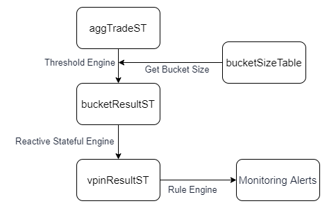
Figure 19. Figure 4-1: Real-Time Streaming Monitoring Workflow - Subscribe to the data separately, feed it into the streaming engines, and compute the results in real time.
Usage:
The following section explains how to use this real-time streaming monitoring
solution. For the complete code, see the attached calcRealTimeTradeVPIN.dos
file.
- Install and load the httpClient plugin, and update the Enterprise WeChat URL in
the monitoring function
sendWechatin the script;installPlugin("httpClient") loadPlugin("httpClient") //Line 117 of the attached script: webhook = "..." - Modify the relevant parameters in the script, such as the trading pair
sym, window sizewindowSize, and monitoring threshold;//Lines 143-150 of the attached script: sym = "BTCUSDT" symSource = "OKX-Futures" windowSize= 5 y = [[<VPIN > 0.2>]] //Trigger an alert when the VPIN value exceeds 0.2 - Place the
calcRealTimeTradeVPIN.dosscript on the server and record its storage path; - Configure a daily scheduled task to recreate the streaming framework;
//scheduleTime uses the current machine's system time and must be adjusted to UTC time scheduleJob(jobId=`calcRealTimeVPIN,jobDesc="calc VPIN daily",jobFunc=run{"calcRealTimeTradeVPIN.dos"}, scheduleTime=00:00m, startDate=2026.01.01, endDate=2036.12.31, frequency='D'); - Because the daily bucket size is based on the average trading volume over the previous N trading days, the streaming engine environment must be recreated each day.
- The sample script sends alerts through Enterprise WeChat.
Real-Time Result Example:
Using real-time aggregated trade data aggTradeST for the BTCUSDT
trading pair, the following example shows the calculation results with a window size
of 5:

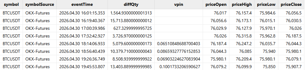
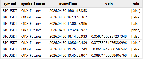
As shown in the figures, bucketResultST is the result table of the
threshold engine and partitions buckets based on bucket size.
VPINResultST is the result table of the reactive stateful engine
and uses the sliding average of diffQty over a window of 5 as the
VPIN value. VPINRuleResultST is the result table of the rule
engine; its last column indicates whether the alert threshold has been exceeded. If
the value is true, an alert message is sent to Enterprise WeChat, email, or another
notification channel.
Replay Historical Data:
Replay the historical aggregated trade data from October 10, 2025 to simulate real-time VPIN calculation and monitoring alerts. The data file is provided in the attached tradeData.zip, and the replay script is provided in the attached replay.dos.
Using the ADAUSDT trading pair as an example, the replay produces the following VPIN result table:
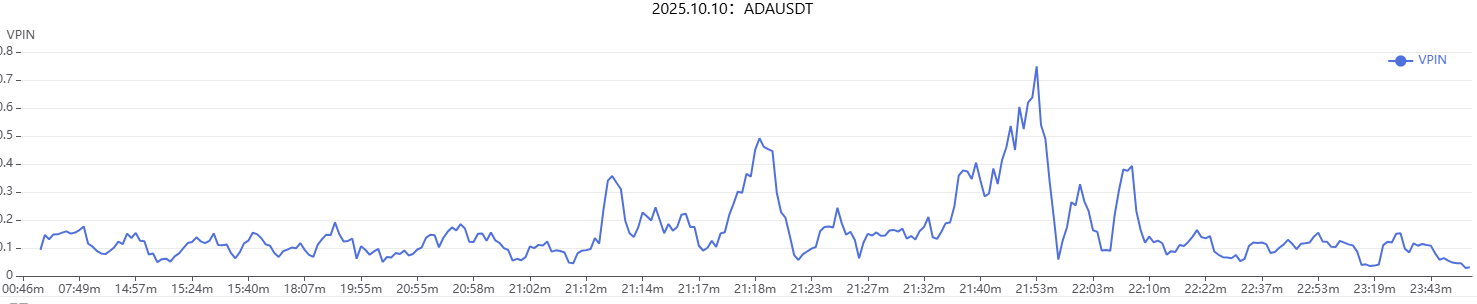
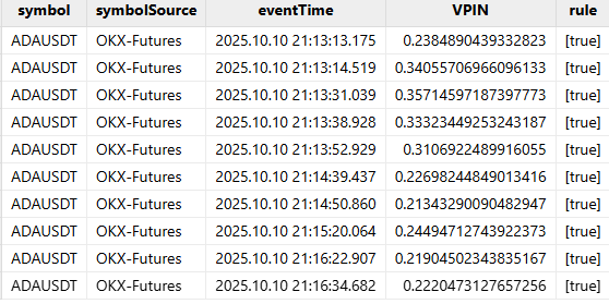
As shown above, Figure 4-5 indicates that the VPIN value increased between 21:00 and 22:10 on that day, corresponding to sharp price fluctuations during the same period. This suggests that the indicator can, to some extent, provide effective risk-control alerts.
5. Summary
This article focuses on price wicking in cryptocurrency markets. It introduces the theoretical background and definition of price wicking, and examines the application of the VPIN indicator and the order book imbalance indicator in analyzing extreme price movements. Using the DolphinDB language, this article implements the corresponding historical indicator calculation modules and a real-time streaming monitoring solution. These components can be applied directly to historical indicator research, real-time market monitoring, and risk-control alerting, providing practical guidance for identifying abnormal volatility and preventing risk in cryptocurrency markets. In addition, this article further analyzes changes in liquidation data, order book depth, and trading volume during the representative event on October 10, 2025. It also uses real-world data, together with the VPIN and order book imbalance indicators, to evaluate their ability to identify price wicking risk.
6. Attachments and References
Attachments
Chapter 3
Chapter 4
Data files (all use UTC time)
References:
[1] ParvezMayar (2025). When Systems Bend but Don't Break: Dolomite's Liquidation & Health Factor Design | ParvezMayar on Binance Square: When Systems Bend but Don't Break: Dolomite's Liquidation & Health Factor Design | ParvezMayar on Binance Square.
[2] Nison, S. (1991). Japanese Candlestick Charting Techniques. New York: New York Institute of Finance.
[3] Torben G. Andersen, Oleg Bondarenko (2014). VPIN and the Flash Crash: Journal of Financial Markets.
[4] How to Read and Interpret Liquidity and Order Book Depth: How to Read and Interpret Liquidity and Order Book Depth.
[5] Jung Hua Liu. (2025). Crypto "Black Swan" Crash: An Academic Analysis: The October 11, 2025 Crypto "Black Swan" Crash: An Academic Analysis | by Jung-Hua Liu | Medium.