
Depth Imbalance, Buy/Sell Pressure, and Realized Volatility Calculation
In financial data analysis, the quality of data preprocessing and feature engineering often determines the efficacy of mathematical models in real-world applications. Certain financial indicators require complex computations across numerous high-dimensional columns in large volumes of raw data, incurring substantial computational costs and development overhead. Using Level-2 snapshot data of securities trading, this tutorial presents scripts for calculating 10-minute frequency indicators, including depth imbalance, buy/sell pressure, and realized volatility. It is intended as a reference for DolphinDB users developing similar factor calculation scripts, improving development efficiency.
1. Schema of Snapshot Data
Table 1-1 Schema of Snapshot Data
| Field | Description |
|---|---|
| SecurityID | Security ID |
| DateTime | Date and time |
| PreClosePx | Previous closing price |
| OpenPx | Opening price |
| HighPx | High price |
| LowPx | Low price |
| LastPx | Last price |
| TotalVolumeTrade | Total trading volume |
| TotalValueTrade | Total trading amount |
| InstrumentStatus | Trading status |
| BidPrice[10] | Bid prices (top 10) |
| BidOrderQty[10] | Bid volumes (top 10) |
| OfferPrice[10] | Ask prices (top 10) |
| OfferOrderQty[10] | Ask volumes (top 10) |
| ... | ... |
This example uses several fields from snapshot data, including SecurityID, DateTime, BidPrice[10], BidOrderQty[10], OfferPrice[10], and OfferOrderQty[10].
The sample data consists of the SSE 50 Index constituents in 2020:
- Stock
code
601318,600519,600036,600276,601166,600030,600887,600016,601328,601288,
600000,600585,601398,600031,601668,600048,601888,600837,601601,601012,
603259,601688,600309,601988,601211,600009,600104,600690,601818,600703,
600028,601088,600050,601628,601857,601186,600547,601989,601336,600196,
603993,601138,601066,601236,601319,603160,600588,601816,601658,600745
The 2020 snapshot data for 14,460 securities from the Shanghai Stock Exchange (SSE) has been imported into a database, with 174 columns and approximately 2.875 billion records in total. See Importing Data to DolphinDB for data import method.
2. Indicator Definitions
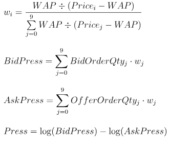
- Weighted Average Price (WAP)

- Depth Imbalance (DI)

- Buy/Sell Pressure (Press)
Feature Data Resampling (10-Minute Windows with Volatility Aggregation)
Resampling with group by SecurityID, interval( TradeTime, 10m, "none"
).
- Realized Volatility (RV)
Realized volatility is defined as the square root of the sum of squared log returns.
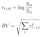
A stock's price always lies between the bid price and ask price. Therefore, this tutorial uses WAP instead of the stock price for calculaion.

3. SQL Optimization
The SQL statement used to calculate these indicators consists of the following parts:
SELECT metric_calculation_function(parameters)
FROM data_source
WHERE date_filter, stock_filter, trading_hours_filter
GROUP BY securityID, interval(temporal_column, time_unit, fill_method)The optimization focuses on the calculation functions of indicators in this tutorial.
Calculation Efficiency
- Total data volume in the DFS table: 2,874,861,174
- Data volume for the SSE 50 Index constituents: 58,257,708
- Data volume in the result table: 267,490
Table 3-1 Calculation Efficiency of Four Implementations
| Implementation | Storage Engine | Storage Schema for 10-Level Bid/Ask Prices and Volumes | Calculate by | Number of CPU Cores | Elapsed Time (s) |
|---|---|---|---|---|---|
| Basic | OLAP | 40 Columns | Column | 8 | 450 |
| Intermediate | OLAP | 40 Columns | Matrix | 8 | 450 |
| Advanced 1 | TSDB | 40 Columns | Matrix | 8 | 27 |
| Advanced 2 | TSDB | 4 Columns (array vector) | Matrix | 8 | 25 |
3.1 Basic: Calculate by Column
The data is stored using the OLAP engine.
Based on the formulas defined in Chapter 2, you can write the following code to calculate by column:
// part1: Define calculation function
def calPress(BidPrice0,BidPrice1,BidPrice2,BidPrice3,BidPrice4,BidPrice5,BidPrice6,BidPrice7,BidPrice8,BidPrice9,BidOrderQty0,BidOrderQty1,BidOrderQty2,BidOrderQty3,BidOrderQty4,BidOrderQty5,BidOrderQty6,BidOrderQty7,BidOrderQty8,BidOrderQty9,OfferPrice0,OfferPrice1,OfferPrice2,OfferPrice3,OfferPrice4,OfferPrice5,OfferPrice6,OfferPrice7,OfferPrice8,OfferPrice9,OfferOrderQty0,OfferOrderQty1,OfferOrderQty2,OfferOrderQty3,OfferOrderQty4,OfferOrderQty5,OfferOrderQty6,OfferOrderQty7,OfferOrderQty8,OfferOrderQty9){
WAP = (BidPrice0*OfferOrderQty0+OfferPrice0*BidOrderQty0)\(BidOrderQty0+OfferOrderQty0)
Bid_1_P_WAP_SUM = 1\(BidPrice0-WAP) + 1\(BidPrice1-WAP) + 1\(BidPrice2-WAP) + 1\(BidPrice3-WAP) + 1\(BidPrice4-WAP) + 1\(BidPrice5-WAP) + 1\(BidPrice6-WAP) + 1\(BidPrice7-WAP) + 1\(BidPrice8-WAP) + 1\(BidPrice9-WAP)
Offer_1_P_WAP_SUM = 1\(OfferPrice0-WAP)+1\(OfferPrice1-WAP)+1\(OfferPrice2-WAP)+1\(OfferPrice3-WAP)+1\(OfferPrice4-WAP)+1\(OfferPrice5-WAP)+1\(OfferPrice6-WAP)+1\(OfferPrice7-WAP)+1\(OfferPrice8-WAP)+1\(OfferPrice9-WAP)
BidPress = BidOrderQty0*((1\(BidPrice0-WAP))\Bid_1_P_WAP_SUM) + BidOrderQty1*((1\(BidPrice1-WAP))\Bid_1_P_WAP_SUM) + BidOrderQty2*((1\(BidPrice2-WAP))\Bid_1_P_WAP_SUM) + BidOrderQty3*((1\(BidPrice3-WAP))\Bid_1_P_WAP_SUM) + BidOrderQty4*((1\(BidPrice4-WAP))\Bid_1_P_WAP_SUM) + BidOrderQty5*((1\(BidPrice5-WAP))\Bid_1_P_WAP_SUM) + BidOrderQty6*((1\(BidPrice6-WAP))\Bid_1_P_WAP_SUM) + BidOrderQty7*((1\(BidPrice7-WAP))\Bid_1_P_WAP_SUM) + BidOrderQty8*((1\(BidPrice8-WAP))\Bid_1_P_WAP_SUM) + BidOrderQty9*((1\(BidPrice9-WAP))\Bid_1_P_WAP_SUM)
OfferPress = OfferOrderQty0*((1\(OfferPrice0-WAP))\Offer_1_P_WAP_SUM) + OfferOrderQty1*((1\(OfferPrice1-WAP))\Offer_1_P_WAP_SUM) + OfferOrderQty2*((1\(OfferPrice2-WAP))\Offer_1_P_WAP_SUM) + OfferOrderQty3*((1\(OfferPrice3-WAP))\Offer_1_P_WAP_SUM) + OfferOrderQty4*((1\(OfferPrice4-WAP))\Offer_1_P_WAP_SUM) + OfferOrderQty5*((1\(OfferPrice5-WAP))\Offer_1_P_WAP_SUM) + OfferOrderQty6*((1\(OfferPrice6-WAP))\Offer_1_P_WAP_SUM) + OfferOrderQty7*((1\(OfferPrice7-WAP))\Offer_1_P_WAP_SUM) + OfferOrderQty8*((1\(OfferPrice8-WAP))\Offer_1_P_WAP_SUM) + OfferOrderQty9*((1\(OfferPrice9-WAP))\Offer_1_P_WAP_SUM)
return log(BidPress)-log(OfferPress)
}
// part2: Define variables and assign values
stockList=`601318`600519`600036`600276`601166`600030`600887`600016`601328`601288`600000`600585`601398`600031`601668`600048`601888`600837`601601`601012`603259`601688`600309`601988`601211`600009`600104`600690`601818`600703`600028`601088`600050`601628`601857`601186`600547`601989`601336`600196`603993`601138`601066`601236`601319`603160`600588`601816`601658`600745
dbName = "dfs://snapshot_SH_L2_OLAP"
tableName = "snapshot_SH_L2_OLAP"
snapshot = loadTable(dbName, tableName)
// part3: Execute SQL
result = select
avg((OfferPrice0\BidPrice0-1)) as BAS,
avg((BidOrderQty0-OfferOrderQty0)\(BidOrderQty0+OfferOrderQty0)) as DI0,
avg((BidOrderQty1-OfferOrderQty1)\(BidOrderQty1+OfferOrderQty1)) as DI1,
avg((BidOrderQty2-OfferOrderQty2)\(BidOrderQty2+OfferOrderQty2)) as DI2,
avg((BidOrderQty3-OfferOrderQty3)\(BidOrderQty3+OfferOrderQty3)) as DI3,
avg((BidOrderQty4-OfferOrderQty4)\(BidOrderQty4+OfferOrderQty4)) as DI4,
avg((BidOrderQty5-OfferOrderQty5)\(BidOrderQty5+OfferOrderQty5)) as DI5,
avg((BidOrderQty6-OfferOrderQty6)\(BidOrderQty6+OfferOrderQty6)) as DI6,
avg((BidOrderQty7-OfferOrderQty7)\(BidOrderQty7+OfferOrderQty7)) as DI7,
avg((BidOrderQty8-OfferOrderQty8)\(BidOrderQty8+OfferOrderQty8)) as DI8,
avg((BidOrderQty9-OfferOrderQty9)\(BidOrderQty9+OfferOrderQty9)) as DI9,
avg(calPress(BidPrice0,BidPrice1,BidPrice2,BidPrice3,BidPrice4,BidPrice5,BidPrice6,BidPrice7,BidPrice8,BidPrice9, BidOrderQty0,BidOrderQty1,BidOrderQty2,BidOrderQty3,BidOrderQty4,BidOrderQty5,BidOrderQty6,BidOrderQty7,BidOrderQty8,BidOrderQty9,OfferPrice0,OfferPrice1,OfferPrice2,OfferPrice3,OfferPrice4,OfferPrice5,OfferPrice6,OfferPrice7,OfferPrice8,OfferPrice9,OfferOrderQty0,OfferOrderQty1,OfferOrderQty2,OfferOrderQty3,OfferOrderQty4,OfferOrderQty5,OfferOrderQty6,OfferOrderQty7,OfferOrderQty8,OfferOrderQty9)) as Press,
sqrt(sum(pow((log((BidPrice0*OfferOrderQty0+OfferPrice0*BidOrderQty0)\(BidOrderQty0+OfferOrderQty0))-prev(log((BidPrice0*OfferOrderQty0+OfferPrice0*BidOrderQty0)\(BidOrderQty0+OfferOrderQty0)))),2))) as RV
from snapshot
where date(TradeTime) between 2020.01.01: 2020.12.31, SecurityID in stockList, (time(TradeTime) between 09:30:00.000: 11:29:59.999) || (time(TradeTime) between 13:00:00.000: 14:56:59.999)
group by SecurityID, interval( TradeTime, 10m, "none" ) as TradeTimeThe code involves 40 columns of data: BidPrice0-9, BidOrderQty0-9, OfferPrice0-9, and OfferOrderQty0-9. The indicator definition is complex. Even after simplification, the code remains lengthy and difficult to modify and maintain.
Calculation Performance
- Total data volume in the DFS table: 2,874,861,174
- Data volume for the SSE 50 Index constituents: 58,257,708
- Logical CPU cores: 8
- Average CPU cores used: 4.5
- Elapsed time: 450s
3.2 Intermediate: Concatenate Columns into a Matrix
The data is stored using the OLAP engine.
The calculations are expressed as column-to-column operations in the formulas defined in Chapter 2. In practice, calculations actually occur across four major groups of columns: BidPrice, BidOrderQty, OfferPrice, and OfferOrderQty (10 columns per group). Therefore, you can treat these four groups as matrices with n rows and 10 columns. You can concatenate the matrices in SQL and then pass them to an aggregate function for matrix operations, as shown in the following example:
// part1: Define calculation function
defg featureEngine(bidPrice,bidQty,offerPrice,offerQty){
 bas = offerPrice[0]\bidPrice[0]-1
 wap = (bidPrice[0]*offerQty[0] + offerPrice[0]*bidQty[0])\(bidQty[0]+offerQty[0])
 di = (bidQty-offerQty)\(bidQty+offerQty)
 bidw=(1.0\(bidPrice-wap))
 bidw=bidw\(bidw.rowSum())
 offerw=(1.0\(offerPrice-wap))
 offerw=offerw\(offerw.rowSum())
 press=log((bidQty*bidw).rowSum())-log((offerQty*offerw).rowSum())
 rv=sqrt(sum2(log(wap)-log(prev(wap))))
 return avg(bas),avg(di[0]),avg(di[1]),avg(di[2]),avg(di[3]),avg(di[4]),avg(di[5]),avg(di[6]),avg(di[7]),avg(di[8]),avg(di[9]),avg(press),rv
}

// part2: Define variables and assign values
stockList=`601318`600519`600036`600276`601166`600030`600887`600016`601328`601288`600000`600585`601398`600031`601668`600048`601888`600837`601601`601012`603259`601688`600309`601988`601211`600009`600104`600690`601818`600703`600028`601088`600050`601628`601857`601186`600547`601989`601336`600196`603993`601138`601066`601236`601319`603160`600588`601816`601658`600745
dbName = "dfs://snapshot_SH_L2_OLAP"
tableName = "snapshot_SH_L2_OLAP"
snapshot = loadTable(dbName, tableName)

// part3: Execute SQL
result1 = select
 featureEngine(
 matrix(BidPrice0,BidPrice1,BidPrice2,BidPrice3,BidPrice4,BidPrice5,BidPrice6,BidPrice7,BidPrice8,BidPrice9),
 matrix(BidOrderQty0,BidOrderQty1,BidOrderQty2,BidOrderQty3,BidOrderQty4,BidOrderQty5,BidOrderQty6,BidOrderQty7, BidOrderQty8,BidOrderQty9),
 matrix(OfferPrice0,OfferPrice1,OfferPrice2,OfferPrice3,OfferPrice4,OfferPrice5,OfferPrice6,OfferPrice7,OfferPrice8, OfferPrice9),
 matrix(OfferOrderQty0,OfferOrderQty1,OfferOrderQty2,OfferOrderQty3,OfferOrderQty4,OfferOrderQty5,OfferOrderQty6, OfferOrderQty7,OfferOrderQty8,OfferOrderQty9)) as `BAS`DI0`DI1`DI2`DI3`DI4`DI5`DI6`DI7`DI8`DI9`Press`RV
 from snapshot
 where date(TradeTime) between 2020.01.01: 2020.12.31, SecurityID in stockList, (time(TradeTime) between 09:30:00.000: 11:29:59.999) || (time(TradeTime) between 13:00:00.000: 14:56:59.999)
 group by SecurityID, interval( TradeTime, 10m, "none" ) as TradeTime map
This matrix-based approach significantly reduces the amount of code required. The calculation logic for indicators is now explicit within the custom aggregate functions, which will greatly facilitate future modifications.
Calculation Performance
- Total data volume in the DFS table: 2,874,861,174
- Data volume for the SSE 50 Index constituents: 58,257,708
- Logical CPU cores: 8
- Average CPU cores used: 4.5
- Elapsed time: 450s
3.3 Advanced 1: Storage and Calculation with TSDB Engine
When creating a DFS database and a partitioned table with the TSDB engine, you must explicitly specify engine and sortColumns. To create the database and table:
dbName = "dfs://snapshot_SH_L2_TSDB"
tableName = "snapshot_SH_L2_TSDB"
dbTime = database(, VALUE, 2020.01.01..2020.12.31)
dbSymbol = database(, HASH, [SYMBOL, 20])
db = database(dbName, COMPO, [dbTime, dbSymbol], engine='TSDB')
createPartitionedTable(dbHandle=db, table=tbTemp, tableName=tableName, partitionColumns=`TradeTime`SecurityID, sortColumns=`SecurityID`TradeTime)
The calculation code is exactly the same as the example in section 3.2.
Data processing performance improves significantly thanks to query optimization of the TSDB storage engine. The calculation took 450 seconds to complete before. After optimization, it takes only 27 seconds, making it 17 times faster than the original version.
Calculation Performance
- Total data volume in the DFS table: 2,874,861,174
- Data volume for the SSE 50 Index constituents: 58,257,708
- Logical CPU cores: 8
- Average CPU core used: 7.6
- Elapsed time without level file index cache: 27s
- Elapsed time with level file index cache: 16s
3.4 Advanced 2: Use Array Vectors for Storage and Calculation with TSDB Engine
Starting with DolphinDB version 2.00.4, DFS tables support storing array vectors. Therefore, when storing data, you can store the 40 columns of BidPrice0-9, BidOrderQty0-9, OfferPrice0-9, and OfferOrderQty0-9 as 4 columns of BidPrice, BidOrderQty, OfferPrice, and OfferOrderQty in an array vector.
// part1: Define calculation function
defg featureEngine(bidPrice,bidQty,offerPrice,offerQty){
 bas = offerPrice[0]\bidPrice[0]-1
 wap = (bidPrice[0]*offerQty[0] + offerPrice[0]*bidQty[0])\(bidQty[0]+offerQty[0])
 di = (bidQty-offerQty)\(bidQty+offerQty)
 bidw=(1.0\(bidPrice-wap))
 bidw=bidw\(bidw.rowSum())
 offerw=(1.0\(offerPrice-wap))
 offerw=offerw\(offerw.rowSum())
 press=log((bidQty*bidw).rowSum())-log((offerQty*offerw).rowSum())
 rv=sqrt(sum2(log(wap)-log(prev(wap))))
 return avg(bas),avg(di[0]),avg(di[1]),avg(di[2]),avg(di[3]),avg(di[4]),avg(di[5]),avg(di[6]),avg(di[7]),avg(di[8]),avg(di[9]),avg(press),rv
}

// part2: Define variables and assign values
stockList=`601318`600519`600036`600276`601166`600030`600887`600016`601328`601288`600000`600585`601398`600031`601668`600048`601888`600837`601601`601012`603259`601688`600309`601988`601211`600009`600104`600690`601818`600703`600028`601088`600050`601628`601857`601186`600547`601989`601336`600196`603993`601138`601066`601236`601319`603160`600588`601816`601658`600745
dbName = "dfs://snapshot_SH_L2_TSDB_ArrayVector"
tableName = "snapshot_SH_L2_TSDB_ArrayVector"
snapshot = loadTable(dbName, tableName)

// part3: Execute SQL
result = select
 featureEngine(BidPrice,BidOrderQty,OfferPrice,OfferOrderQty) as `BAS`DI0`DI1`DI2`DI3`DI4`DI5`DI6`DI7`DI8`DI9`Press`RV
 from snapshot
 where date(TradeTime) between 2020.01.01: 2020.12.31, SecurityID in stockList, (time(TradeTime) between 09:30:00.000: 11:29:59.999) || (time(TradeTime) between 13:00:00.000: 14:56:59.999)
 group by SecurityID, interval( TradeTime, 10m, "none" ) as TradeTime map
Using array vectors for data storage does not significantly improve performance compared to column-by-column storage, but it does make the code more concise and easier to modify and maintain.
Calculation Performance
- Total data volume in the DFS table: 2,874,861,174
- Data volume for the SSE 50 Index constituents: 58,257,708
- Logical CPU cores: 8
- Average CPU core used: 7.6
- Elapsed time without level file index cache: 25s
- Elapsed time with level file index cache: 15s
4. Reasons for the Performance Improvement from OLAP to TSDB
4.1 Database Creation
Code for creating a DFS database with the OLAP engine:
dbName = "dfs://snapshot_SH_L2_OLAP"
dbTime = database(, VALUE, 2020.01.01..2020.12.31)
dbSymbol = database(, HASH, [SYMBOL, 20])
db = database(dbName, COMPO, [dbTime, dbSymbol])
Code for creating a DFS database with the TSDB engine:
dbName = "dfs://snapshot_SH_L2_TSDB"
dbTime = database(, VALUE, 2020.01.01..2020.12.31)
dbSymbol = database(, HASH, [SYMBOL, 20])
db = database(dbName, COMPO, [dbTime, dbSymbol], engine='TSDB')
In DolphinDB, partitioning rules are defined at the database level. In this example, the OLAP and TSDB engines use the same partitioning rules: data is first partitioned by day and then hash-partitioned by security ID into 20 partitions. As a result, the daily data for 14,460 securities is distributed relatively evenly across 20 partitions, and the data for the SSE 50 Index constituents is also spread across multiple partitions. Each partition contains data for multiple securities that share the same hash value.
The OLAP and TSDB engines use the same data partitioning algorithm. Therefore, in this example, the only difference in database creation is that the TSDB engine requires the engine parameter to be set to TSDB, whose default value is OLAP.
4.2 Table Creation
Code for creating a partitioned DFS table with the OLAP engine:
dbName = "dfs://snapshot_SH_L2_OLAP"
db = database(dbName)
tableName = "snapshot_SH_L2_OLAP"
createPartitionedTable(dbHandle=db, table=tbTemp, tableName=tbName, partitionColumns=`TradeTime`SecurityID)
Code for creating a partitioned DFS table with the TSDB engine:
dbName = "dfs://snapshot_SH_L2_TSDB"
db = database(dbName)
tableName = "snapshot_SH_L2_TSDB"
createPartitionedTable(dbHandle=db, table=tbTemp, tableName=tableName, partitionColumns=`TradeTime`SecurityID, sortColumns=`SecurityID`TradeTime)
In the preceding example, a partitioned DFS table is created in the TSDB database
with sortColumns set to `SecurityID`TradeTime.
sortColumns generally consists of two parts:
- sortKey: One or more query index columns, excluding the temporal column.
- Temporal column: The temporal column in the data, used to sort data within each partition in chronological order.
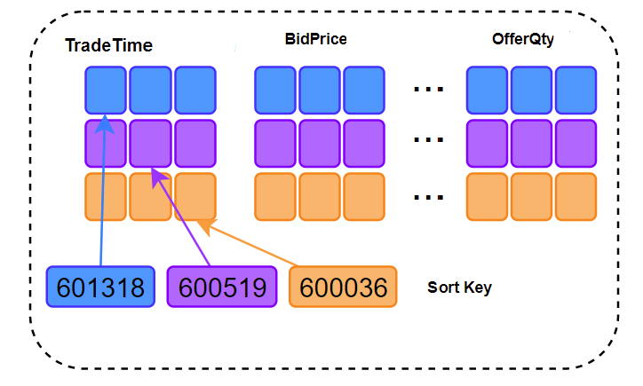
In this example, sortKey is SecurityID, and the temporal column is TradeTime. Compared with the OLAP engine, the TSDB engine stores the data for each SecurityID contiguously within each partition's disk files, and the data is strictly ordered by TradeTime. Besides, when the TSDB engine filters and queries data by sortColumns, it can use index files within a partition to load only the data that meets the filters from disk.
The calculation sample in this tutorial is the SSE 50 Index constituents in 2020, and the data source is the SSE data for all 14,460 securities in 2020. If you use the OLAP engine, data for unrelated securities in the relevant partitions must be loaded from disk to memory before decompression, filtering, and calculation. If you use TSDB, only the data for the SSE 50 Index constituents needs to be loaded from disk into memory for calculation.
4.3 Differences Between the OLAP and TSDB Engines
The OLAP engine preserves write order and stores data to disk in an append-only manner. In a partitioned DFS table, each column in each partition is stored as a separate file. For a given column file, data for multiple SecurityID values is appended in write order, so data for the same SecurityID is possibly scattered across the column file. In this example, the queried table stores data for 14,460 securities. Although only data for the SSE 50 Index constituents is queried, data for unrelated securities in the relevant partitions is also read from disk into memory for decompression when using the OLAP engine, which reduces data retrieval efficiency.
Data for the same SecurityID is stored contiguously and compressed during storage if you set sortColumns=`SecurityID`TradeTime.
- If all data for the same SecurityID is compressed together, even if you need only a small subset of that SecurityID data when querying, all of it must still be read from disk into memory for decompression, reducing the query efficiency.
- Therefore, the TSDB engine compresses and stores all data for the same SecurityID within the same level file, while associating it with a time range for query. The data within that time range represents only a small subset of all data for that SecurityID. In this example, data for the same SecurityID is ordered by sortColumns, whose last column is TradeTime, and is then stored in data blocks of a certain size (16 KB by default). When reading data, TSDB first uses the stock column and temporal column as filter conditions in the query to quickly locate the data blocks that meet the filter conditions. Then only those blocks are loaded into memory for decompression. These blocks usually account for only a small portion of the total data, greatly improving the query efficiency.
4.4 Chapter Summary
In this tutorial, the TSDB engine delivers better performance than the OLAP engine for the following main reasons:
- In this tutorial, the queried table stores all Level-2 snapshot data for SSE in 2020 with a total of 2,874,861,174 records for 14,460 securities. The sample data used in the calculation consists of the SSE 50 Index constituents in 2020, with a total of 58,257,708 records. Without any caching, the TSDB engine needs to read only 58,257,708 records from disk compared to OLAP engine.
- Starting from version 2.00.4, DolphinDB supports storing array vectors in DFS tables. This is particularly well suited to storing multi-level bid/ask price and volume data in snapshots. For SSE Level-2 snapshot data, the compression ratio can reach 9~11 using array vectors. Without any caching, using array vectors increases the number of records that can be read from disk per unit time compared with multi-column storage.
- By storing the multi-level bid/ask price and volume data in Level-2 snapshot data as array vectors in the TSDB engine, the data is stored as a vector in a specific row and column of a DFS table. As a result, when you perform matrix operations on multi-level bid/ask price and volume data, retrieving multiple rows from a single column returns a matrix directly. Compared with a multi-column storage, this approach eliminates the need for matrix concatenation.
5. Summary
For the same scenario, this example provides four SQL implementations:
- The Basic version uses the OLAP engine and a column-oriented approach. It is easy to develop, but the code is lengthy and difficult to modify. Elapsed time is 450 seconds.
- The Intermediate version uses the OLAP engine and a matrix-based approach. It is moderately difficult to develop, requires less code, and expresses the computational logic more clearly. Elapsed time is 450 seconds.
- The Advanced 1 version uses the TSDB engine and a matrix-based approach. The script is exactly the same as in the intermediate version. Elapsed time is 27 seconds without the level file index cache and 16 seconds with the level file index cache.
- The Advanced 2 version uses the TSDB engine, with the multi-level bid/ask price and volume data stored as array vectors. It also follows a matrix-based approach. The code is more concise, making later modification and maintenance easier. Elapsed time is 25 seconds without the level file index cache and 15 seconds with the level file index cache.
This tutorial aims to provide DolphinDB users with an example for developing similar factor calculation scripts, improving development efficiency.