Calculating OHLC bars
OHLC bars can be efficiently calculated in various scenarios in DolphinDB. This tutorial will introduce how to calculate OHLC bars with historical data and real-time data.
With Historical Data
We will explain how to calculate OHLC bars with batch calculation for the following scenarios:
the starting time of the OHLC windows need to specified;
multiple trading sessions in a day, including overnight sessions;
overlapping OHLC windows; OHLC windows deliminated based on trading volume.
If there is a very large amount of data, and the results need to be written to the database, we can use the built-in Map-Reduce function in DolphinDB for parallel computing.
With Real-time Data
Use APIs to receive market data in real time, and use DolphinDB's built-in time-series engine for real-time calculation.
1. Calculation with Historical Data (Batch Calculation)
To calculate OHLC bars with historical data, you can use DolphinDB's built-in functions bar, dailyAlignedBar or wj.
1.1. Without Specifying the Starting Time of OHLC Windows
Function bar is generally used to group data based on specified interval.
date = 09:32m 09:33m 09:45m 09:49m 09:56m 09:56m;
bar(date, 5);
The result is:
[09:30m,09:30m,09:45m,09:45m,09:55m,09:55m]Example 1:
n = 1000000
date = take(2019.11.07 2019.11.08, n)
time = (09:30:00.000 + rand(int(6.5*60*60*1000), n)).sort!()
timestamp = concatDateTime(date, time)
price = 100+cumsum(rand(0.02, n)-0.01)
volume = rand(1000, n)
symbol = rand(`AAPL`FB`AMZN`MSFT, n)
trade = table(symbol, date, time, timestamp, price, volume).sortBy!(`symbol`timestamp)
undef(`date`time`timestamp`price`volume`symbol);
Calculate 5-minute OHLC bars:
barMinutes = 5m
OHLC = select first(price) as open, max(price) as high, min(price) as low, last(price) as close, sum(volume) as volume from trade group by symbol, date, bar(time, barMinutes) as barStart
Parameter interval of function bar supports the DURATION type. "5m" here means 5 minutes.
1.2. Specifying the Starting Time of OHLC Windows
Use function dailyAlignedBar to specify the starting time of OHLC windows. This function can accommodate multiple trading sessions per day as well as overnight sessions.
Note that for function dailyAlignedBar, the data type of the temporal column can be SECOND, TIME, NANOTIME, DATETIME, TIMESTAMP and NANOTIMESTAMP. The parameter 'timeOffset' that specifies the starting time of each trading session must have the corresponding data type: SECOND, TIME or NANOTIME, respectively.
Example 2 (one trading session per day): Calculate 7-minute OHLC bars with the same table 'trade' in Example 1.
barMinutes = 7m
OHLC = select first(price) as open, max(price) as high, min(price) as low, last(price) as close, sum(volume) as volume from trade group by symbol, dailyAlignedBar(timestamp, 09:30:00.000, barMinutes) as barStart
Example 3 (two trading sessions per day): China's stock market has two trading sessions per day, from 9:30 to 11:30 in the morning and from 13:00 to 15:00 in the afternoon.
Use the following script to generate simulated data:
n = 1000000
date = take(2019.11.07 2019.11.08, n)
time = (09:30:00.000 + rand(2*60*60*1000, n/2)).sort!() join (13:00:00.000 + rand(2*60*60*1000, n/2)).sort!()
timestamp = concatDateTime(date, time)
price = 100+cumsum(rand(0.02, n)-0.01)
volume = rand(1000, n)
symbol = rand(`600519`000001`600000`601766, n)
trade = table(symbol, timestamp, price, volume).sortBy!(`symbol`timestamp)
undef(`date`time`timestamp`price`volume`symbol)
Calculate the 7-minute OHLC bars:
barMinutes = 7m
sessionsStart=09:30:00.000 13:00:00.000
sessionsEnd=11:30:00.000 15:00:00.000
OHLC = select first(price) as open, max(price) as high, min(price) as low, last(price) as close, sum(volume) as volume from trade group by symbol, dailyAlignedBar(timestamp, sessionsStart, barMinutes, sessionsEnd) as barStart
Example 4 (two trading sessions per day with an overnight session): Some futures have multiple trading sessions per day including an overnight session. In this example, the first trading session is from 8:45 AM to 13:45 PM, and the other session is an overnight session from 15:00 PM to 05:00 AM the next day.
Use the following script to generate simulated data:
daySession =  08:45:00.000 : 13:45:00.000
nightSession = 15:00:00.000 : 05:00:00.000
n = 1000000
timestamp = rand(concatDateTime(2019.11.06, daySession[0]) .. concatDateTime(2019.11.08, nightSession[1]), n).sort!()
price = 100+cumsum(rand(0.02, n)-0.01)
volume = rand(1000, n)
symbol = rand(`A120001`A120002`A120003`A120004, n)
trade = select * from table(symbol, timestamp, price, volume) where timestamp.time() between daySession or timestamp.time()>=nightSession[0] or timestamp.time()<nightSession[1] order by symbol, timestamp
undef(`timestamp`price`volume`symbol);
Calculate the 7-minute OHLC bars:
barMinutes = 7m
sessionsStart = [daySession[0], nightSession[0]]
OHLC = select first(price) as open, max(price) as high, min(price) as low, last(price) as close, sum(volume) as volume from trade group by symbol, dailyAlignedBar(timestamp, sessionsStart, barMinutes) as barStart
1.3. Overlapping OHLC Windows
In the examples above, the OHLC windows do not overlap. To calculate overlapping OHLC windows, you can use function wj. With the wj function, each row in the left table corresponds to a window in the right table, and calculations can be conducted on this window.
Example 5. 2 trading sessions per day with overlapping OHLC windows
Simulate Chinese stock market data and calculate a 30-minute OHLC bars every 5 minutes.
n = 1000000
sampleDate = 2019.11.07
symbols = `600519`000001`600000`601766
trade = table(take(sampleDate, n) as date,
	(09:30:00.000 + rand(7200000, n/2)).sort!() join (13:00:00.000 + rand(7200000, n/2)).sort!() as time,
	rand(symbols, n) as symbol,
	100+cumsum(rand(0.02, n)-0.01) as price,
	rand(1000, n) as volume)
First generate OHLC windows, then use function cj(cross join) to generate a combination of stock symbols and OHLC windows.
barWindows = table(symbols as symbol).cj(table((09:30:00.000 + 0..23 * 300000).join(13:00:00.000 + 0..23 * 300000) as time))Then use function wj to calculate OHLC bars with overlapping windows:
OHLC = wj(barWindows, trade, 0:(30*60*1000),
		<[first(price) as open, max(price) as high, min(price) as low, last(price) as close, sum(volume) as volume]>, `symbol`time)
1.4. Determine Windows with Trading Volume
The windows in all of the examples above were determined with time. You can use other variables such as trading volume as the basis to determine windows.
Example 6: OHLC bars are calculated every time trading volume increases by 1,000,000.
n = 1000000
sampleDate = 2019.11.07
symbols = `600519`000001`600000`601766
trade = table(take(sampleDate, n) as date,
	(09:30:00.000 + rand(7200000, n/2)).sort!() join (13:00:00.000 + rand(7200000, n/2)).sort!() as time,
	rand(symbols, n) as symbol,
	100+cumsum(rand(0.02, n)-0.01) as price,
	rand(1000, n) as volume)

volThreshold = 1000000
t = select first(time) as barStart, first(price) as open, max(price) as high, min(price) as low, last(price) as close, last(cumvol) as cumvol
from (select symbol, time, price, cumsum(volume) as cumvol from trade context by symbol)
group by symbol, bar(cumvol, volThreshold) as volBar;
1.5. Use Map-Reduce to Speed up Calculation
If you need to extract large-scale historical data from the database, calculate OHLC bars, and then save them into the database, we can use the built-in MapReduce function mr for parallel loading and calculation. This method can significantly increase speed.
This example uses US stock market trading data. The raw data is stored in table 'trades' in database "dfs://TAQ" with a composite partition: a value partition based on trading dates and a range partition based on stock symbols.
(1) Load the metadata of the table on disk into memory:
login(`admin, `123456)
db = database("dfs://TAQ")
trades = db.loadTable("trades")
(2) Create a template table 'model', then create an empty table 'OHLC' in database "dfs://TAQ" based on the schema of the template table to store the results:
model=select top 1 Symbol, Date, Time.second() as bar, PRICE as open, PRICE as high, PRICE as low, PRICE as close, SIZE as volume from trades where Date=2007.08.01, Symbol=`EBAY
if(existsTable("dfs://TAQ", "OHLC"))
	db.dropTable("OHLC")
db.createPartitionedTable(model, `OHLC, `Date`Symbol)
(3) Use function mr to calculate OHLC bars and write the results to table 'OHLC':
def calcOHLC(inputTable){
	tmp=select first(PRICE) as open, max(PRICE) as high, min(PRICE) as low, last(PRICE) as close, sum(SIZE) as volume from inputTable where Time.second() between 09:30:00 : 15:59:59 group by Symbol, Date, 09:30:00+bar(Time.second()-09:30:00, 5*60) as bar
	loadTable("dfs://TAQ", `OHLC).append!(tmp)
	return tmp.size()
}
ds = sqlDS(<select Symbol, Date, Time, PRICE, SIZE from trades where Date between 2007.08.01 : 2019.08.01>)
mr(ds, calcOHLC, +)- 'ds' is a series of data sources generated by function
sqlDS. Each data source represents data from a partition. - Function
calcOHLCis the map function in MapReduce. It calculates OHLC bars from each data source, writes the result to the database and returns the number of rows written to the database. - "+" is the reduce function in MapReduce. It adds up the results of all map functions (the number of rows written to the database) to return the total number of rows written to the database.
2. Real-time Calculation
The following figure describes the process of calculating OHLC bars in real-time in DolphinDB:
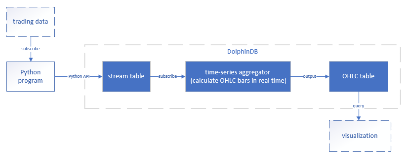
Data vendors usually provide subscription services with on APIs in Python, Java or other languages. In this example, trading data is written into a stream table through DolphinDB Python API. DolphinDB's time-series engine conducts real-time OHLC calculations at specified frequencies.
This example uses the text file trades.csv to simulate real-time data. The following table shows its column names and one row of sample data:
| Symbol | Datetime | Price | Volume |
|---|---|---|---|
| 000001 | 2018.09.03T09:30:06 | 10.13 | 4500 |
The output table for calculation results contains the following 7 columns:
| datetime | symbol | open | close | high | low | volume |
|---|---|---|---|---|---|---|
| 2018.09.03T09:30:07 | 000001 | 10.13 | 10.13 | 10.12 | 10.12 | 468060 |
The following sections describe the steps of real-time calculation of OHLC bars:
2.1. Use Python to Receive Real-time Data and Write to DolphinDB Stream Table
- Create a stream table in DolphinDB
share streamTable(100:0, `Symbol`Datetime`Price`Volume,[SYMBOL,DATETIME,DOUBLE,INT]) as Trade- Insert simulated data to the stream table
As the unit of column 'Datetime' is SECOND and DataFrame in pandas can only use DateTime[64] which corresponds to nanotimestamp data type in DolphinDB, we need to convert the data type of column 'Datetime' before inserting the data to the stream table.
import dolphindb as ddb
import pandas as pd
import numpy as np
csv_file = "trades.csv"
csv_data = pd.read_csv(csv_file, dtype={'Symbol':str} )
csv_df = pd.DataFrame(csv_data)
s = ddb.session();
s.connect("127.0.0.1",8848,"admin","123456")

# Upload DataFrame to DolphinDB and convert the data type of column 'Datetime'

s.upload({"tmpData":csv_df})
s.run("data = select Symbol, datetime(Datetime) as Datetime, Price, Volume from tmpData")
s.run("tableInsert(Trade,data)")
2.2. Calculate OHLC Bars in Real Time
OHLC bars can be calculated in moving windows in real time in DolphinDB. Generally there are the following two scenarios:
Calculations are conducted after windows end
- Nonoverlapping windows
- Partially overlapping windows
Calculations are conducted continuously within the current window
2.2.1. Calculations Are Conducted After Windows End
For nonoverlapping windows, set the same value for parameter 'windowSize' and parameter 'step' of function createTimeSeriesEngine. For overlapping windows, set 'windowSize'>'step'. Please note that 'windowSize' must be a multiple of 'step'.
Non-overlapping windows: calculate OHLC bars for the previous 5 minutes every 5 minutes.
share streamTable(100:0, `datetime`symbol`open`high`low`close`volume,[DATETIME,SYMBOL,DOUBLE,DOUBLE,DOUBLE,DOUBLE,LONG]) as OHLC1
tsEngine1 = createTimeSeriesEngine(name="tsEngine1", windowSize=300, step=300, metrics=<[first(Price),max(Price),min(Price),last(Price),sum(volume)]>, dummyTable=Trade, outputTable=OHLC1, timeColumn=`Datetime, keyColumn=`Symbol)
subscribeTable(tableName="Trade", actionName="act_tsEngine1", offset=0, handler=append!{tsEngine1}, msgAsTable=true);
Overlapping windows: calculate OHLC bars for the previous 5 minutes every 1 minute.
share streamTable(100:0, `datetime`symbol`open`high`low`close`volume,[DATETIME,SYMBOL,DOUBLE,DOUBLE,DOUBLE,DOUBLE,LONG]) as OHLC2
tsEngine2 = createTimeSeriesEngine(name="tsEngine2", windowSize=300, step=60, metrics=<[first(Price),max(Price),min(Price),last(Price),sum(volume)]>, dummyTable=Trade, outputTable=OHLC2, timeColumn=`Datetime, keyColumn=`Symbol)
subscribeTable(tableName="Trade", actionName="act_tsEngine2", offset=0, handler=append!{tsEngine2}, msgAsTable=true);
2.2.2. Multiple Calculations Within a Window
If 'updateTime' is not specified, calculation for a window will not occur before the ending time of the window. To conduct calculations for the current window before it ends, we can specify 'updateTime'. 'step' must be a multiple of 'updateTime'.
If 'updateTime' is specified, multiple calculations may happen within the current window. These calculations are triggered with the following rules:
(1) Divide the current window into 'windowSize'/'updateTime' small windows. Each small window has a length of 'updateTime'. When a new record arrives after a small window finishes, if there is at least one record in the current window that is not used in a calculation (excluding the new record), a calculation is triggered. Please note that this calculation does not use the new record.
(2) If max(2*updateTime, 2 seconds) after a record arrives at the aggregator, it still has not been used in a calculation, a calculation is triggered. This calculation includes all data in the current window at the time.
If 'keyColumn' is specified, these rules apply within each group.
The timestamp of each calculation result within the current window is the current window starting time or starting time + 'windowSize' (depending on parameter 'useWindowStartTime') instead of a timestamp inside the current window.
If 'updateTime' is specified, 'outputTable' must be a keyed table (created with function keyedTable).
In the following example, we calculate 1-minute OHLC bars. Calculations for the current window are triggered no later than 2 seconds after a new message arrives.
First, create a keyed stream table as the output table and use columns 'datetime' and 'Symbol' as primary keys.
share keyedTable(`datetime`Symbol, 100:0, `datetime`Symbol`open`high`low`close`volume,[DATETIME,SYMBOL,DOUBLE,DOUBLE,DOUBLE,DOUBLE,LONG]) as OHLCIn the time-series aggregator, parameter 'updateTime' is set to 1 (second); parameter 'useWindowStartTime' is set to true which means the first column of the output table is the starting time of the windows.
tsEngine = createTimeSeriesEngine(name="tsEngine", windowSize=60, step=60, metrics=<[first(Price),max(Price),min(Price),last(Price),sum(volume)]>, dummyTable=Trade, outputTable=OHLC, timeColumn=`Datetime, keyColumn=`Symbol, updateTime=1, useWindowStartTime=true)Subscribe to the stream table "Trade":
subscribeTable(tableName="Trade", actionName="act_tsEngine", offset=0, handler=append!{tsEngine}, msgAsTable=true);2.3. Display OHLC Bars in Python
In this example, the output table of the aggregator is also defined as a stream table. The client can subscribe to the output table through Python API and display the calculation results to the Python terminal.
The following script uses Python API to subscribe to the output table OHLC of the real-time aggregation calculation, and print the result.
from threading import Event
import dolphindb as ddb
import pandas as pd
import numpy as np
s = ddb.session()
# set local port 20001 for subscribed streaming data
s.enableStreaming(20001)
def handler(lst):
    print(lst)
# subscribe to the stream table OHLC (local port 8848)
s.subscribe ("127.0.0.1", 8848, handler, "OHLC")
Event().Wait()
You can also connect to DolphinDB database through a data visualization tool such as Grafana to query the output table and display the results in charts.