Portfolio Optimization: A Guide to DolphinDB Optimization Solvers
Linear and nonlinear programming are fundamental to operations research, with broad applications in finance and economics. In quantitative finance, portfolio optimization is essential to multi-factor models. It consists of two key components: the objective function and its corresponding constraints. The objective function may aim to maximize expected returns, minimize portfolio risk, or maximize utility. These objectives are subject to various equality and inequality constraints that define the feasible solution space. These optimization problems illustrate the practical use of linear and nonlinear programming.
Portfolio optimization in multi-factor quantitative investment strategies aims to determine optimal asset weights through tactical asset allocation (TAA), with risk control as a primary consideration. The strategy integrates an alpha model with a risk model, which can be demonstrated through the Mean-Variance Optimization (MVO) framework developed by Markowitz in 1952. Assume:
 is the target active weight vector for n stocks, where
 is the expected return vector obtained from the alpha model
- Σ is the covariance matrix of returns
The general framework for MVO is as follows:
Objective Function:

Constraints:
- Weight relationship:

- Tracking error:

- Turnover:

- Weight boundaries:

- Risk factor exposures:

- Number of stocks:

Where, ω represents the target absolute weight vector for n stocks, ω0 is the initial weight vector for the stocks, ωβ denotes the benchmark portfolio weight vector, and λ is the coefficient for the aversion to transaction costs.
DolphinDB addresses various optimization scenarios through specialized solver functions designed for practical applications. The implementation process follows a structured approach:
- Analyze business requirements.
- Identify the key elements of the optimization problem: decision variables, objective function, and constraints.
- Establish the appropriate mathematical programming model.
- Import the model into the solver for optimization.
This tutorial demonstrates how to use DolphinDB optimization solvers, covering both theoretical optimization models and their practical application to portfolio optimization problems.
1. Introduction to Optimization Solvers
DolphinDB provides multiple optimization solvers to address various optimization problems under different constraints.
1.1 Linear Programming (linprog)
The linprog function solves optimization problems with linear objective functions and linear constraints.
Mathematical Model

In this model:
- x is the unknown variable, often referred to as the decision variable in optimization problems.
- min denotes minimization of fTx with respect to x.
- Expressions in the braces after
such thatrepresent equality and inequality constraints.
All relationships in this formulation—both the objective function and constraints—must be linear to qualify as a linear programming (LP) problem.
For cases requiring maximization rather than minimization, the objective function can be transformed by multiplying it by -1.
1.2 Quadratic Programming (quadprog)
The quadprog function solves optimization problems with quadratic objective functions subject to linear constraints.
Mathematical Model

H must be a symmetric positive-definite matrix.
Compared to linear programming, this model's objective function includes an additional quadratic term for x.
1.3 Quadratically Constrained Linear Programming (qclp)
The qclp function solves optimization problems with linear objective functions subject to quadratic constraints.
Mathematical Model
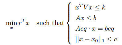
Compared to linear programming, this model introduces non-linear inequality constraints and absolute-valued vector inequality constraint.
1.4 Second-Order Cone Programming (socp)
The socp function implements second-order cone programming (SOCP), offering a more general optimization framework that aligns with the ECOS solver method used in Python's cvxpy library.
Mathematical Model
Definition of k-dimensional standard cone:

The SOCP model uses the Euclidean norm (L2 norm):

Cone representation:
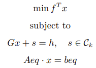
Where Ck denotes the cone and s is a slack variable. In practical
socp function usage, s is determined during
optimization.
Standard form of SOCP:
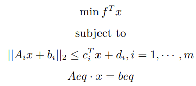
Where  is the cone constraint.
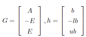
The transformation between cone and standard forms involves specific matrix G and vector h constructions where:
- Matrix G:

- Vector h:

1.5 Gurobi Plugin
The gurobi plugin integrates the Gurobi Optimizer with DolphinDB, providing access to Gurobi's powerful optimization capabilities. This integration maintains Gurobi's conventional usage while offering several advantages. The plugin streamlines the optimization workflow by enabling direct computation within DolphinDB, which reduces data transfer overhead and improves computational efficiency. DolphinDB users can leverage their knowledge of DolphinScript to work with the optimizers effectively.
The current implementation supports Gurobi Optimizer version 10.0.2 and can handle Linear Programming (LP), Quadratic Programming (QP), and Quadratically Constrained Linear Programming (QCLP) problems. Detailed usage instructions can be found in User Manual > gurobi plugin.
Important: The performance tests referenced in subsequent sections reflect results obtained using a single-user Gurobi license, which imposes limitations of 2000 variables and constraints.
2. Converting Programming Problems to SOCP Form
The conversion of general programming problems to SOCP requires transforming the original problem into SOCP standard form by constructing appropriate parameters based on the relationship between cone representation and standard form.
2.1 SOCP Form of Linear Programming
For problems with linear inequality constraints Ax ≤ b, we can rearrange terms
for  .
.
For the linear constraints of the variable x, upper and lower bounds lb ≤ ub can be converted to

Standard SOCP form:

Where E is an identity matrix of the same dimension as x.
Construct the parameters:
2.2 SOCP Form of Quadratic Inequality Constraints
For quadratic inequality constraints ![]() where V is a positive definite matrix and k is
a positive scalar. V can be decomposed using Cholesky decomposition into V =
FTF. The original constraint can then be transformed:
where V is a positive definite matrix and k is
a positive scalar. V can be decomposed using Cholesky decomposition into V =
FTF. The original constraint can then be transformed:

Standard SOCP form:

Construct the parameters:

Where n indicates the length of variable x.
2.3 SOCP Form of Absolute Value Constraints
For linear programming problems that involve absolute value constraints

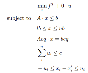
The 1-norm constraints can be expressed as the absolute value constraints.

By introducing auxiliary variable ui

We can rewrite the problem in terms of the vector [xT, u1, ··· , un]T and convert it into the SOCP form.
2.4 SOCP Form of Quadratic Programming
For programming problems with quadratic terms in the objective function, we can introduce an auxiliary variable y = xTHx, where H is a positive definite matrix. Through Cholesky decomposition, H can be decomposed into H = UTU. The problem can be transformed to:

Based on  we can get

Rearranging terms:

Second-order cone constraints:

Standard SOCP form:
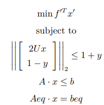
Where

3. Application Scenarios
3.1 Maximizing Expected Returns
In stock portfolio optimization problems, investors seek to maximize portfolio returns while adhering to various constraints. These constraints typically include minimum and maximum allocation limits for individual stocks, risk management parameters, and sector exposure restrictions. Consider a scenario with 10 stocks distributed across three sectors: consumer goods, finance, and technology. The stocks have expected annual returns of 0.1, 0.02, 0.01, 0.05, 0.17, 0.01, 0.07, 0.08, 0.09, 0.10 respectively. The portfolio must maintain sector diversification by limiting exposure to each industry to no more than 8% of the total portfolio value. Additionally, to prevent overconcentration in any single security, the maximum weight allocated to each individual stock cannot exceed 15% of the portfolio.
3.1.1 linprog Solver
Based on the problem description, the linear programming model is defined as follows.
Objective Function: Maximize the portfolio's expected return.

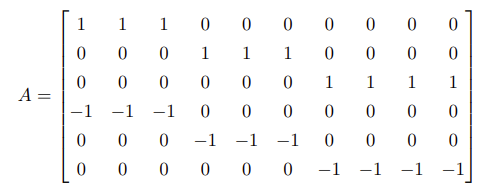
Inequality Constraints:

Equality Constraint:
- The sum of all stock weights = 1.
f = -1*[0.1,0.02,0.01,0.05,0.17,0.01,0.07,0.08,0.09,0.10]
A = ([1,1,1,0,0,0,0,0,0,0,0,0,0,1,1,1,0,0,0,0,0,0,0,0,0,0,1,1,1,1,-1,-1,-1,0,0,0,0,0,0,0,0,0,0,-1,-1,-1,0,0,0,0,0,0,0,0,0,0,-1,-1,-1,-1]$10:6).transpose()
b = [0.3,0.4,0.3]
exposure = 0.08
b = (b + exposure) join (exposure - b)
Aeq = matrix(take(1, size(f))).transpose()
beq = array(DOUBLE).append!(1)
res = linprog(f, A, b, Aeq, beq, 0, 0.15)

max_return = -res[0] // output: 0.0861
weights = res[1] // output: [0.15,0.15,0,0.15,0.15,0.02,0,0.08,0.15,0.15]
3.1.2 Gurobi Plugin
loadPlugin("plugins/gurobi/PluginGurobi.txt")
model = gurobi::model()

// Add variables
numOfVars = 10
lb = take(0, numOfVars)
ub = take(0.15, numOfVars)
stocks = ["A001", "A002", "A003", "A004", "A005", "A006", "A007", "A008", "A009", "A010"]
vars = gurobi::addVars(model, lb, ub, , , stocks)

// Add linear constraints
f = [0.1,0.02,0.01,0.05,0.17,0.01,0.07,0.08,0.09,0.10]
A = ([1,1,1,0,0,0,0,0,0,0,0,0,0,1,1,1,0,0,0,0,0,0,0,0,0,0,1,1,1,1,-1,-1,-1,0,0,0,0,0,0,0,0,0,0,-1,-1,-1,0,0,0,0,0,0,0,0,0,0,-1,-1,-1,-1]$10:6)
rhs = 0.38 0.48 0.38 -0.22 -0.32 -0.22

for (i in 0:6) {
  lhsExpr = gurobi::linExpr(model, A[i], stocks)
  gurobi::addConstr(model, lhsExpr, '<', rhs[i])
}

lhsExpr = gurobi::linExpr(model, take(1, numOfVars), stocks)
gurobi::addConstr(model, lhsExpr, '=', 1)

// Set objective function
obj = gurobi::linExpr(model, f, vars)
gurobi::setObjective(model, obj, -1)

// Solve the optimization
gurobi::optimize(model)

result = gurobi::getResult(model) // stock weights: [0.15,0.15,0,0.15,0.15,0.02,0,0.08,0.15,0.15]
obj = gurobi::getObjective(model) // maximum epected return: 0.0861
3.2 Utility Maximization
Modern portfolio theory (MPT) quantifies investment decisions through the fundamental relationship between returns and risk, using mean return and variance as their respective measures. The utility function represents an investor's preferences by combining these two elements: the desire to maximize expected returns while controlling for portfolio risk. Portfolio optimization typically involves solving a quadratic objective function that incorporates both the expected return and the covariance matrix of returns, reflecting the mathematical expression of this risk-return tradeoff.
Consider a portfolio comprising 2457 stocks where, for simplification, the covariance matrix of returns is assumed to be an identity matrix. The optimization problem seeks to determine the optimal weight allocation across all stocks under these conditions.
3.2.1 quadprog Solver
baseDir = "/home/data/"
f = dropna(flatten(float(matrix(select col1, col2, col3, col4, col5, col6, col7, col8, col9, col10 from loadText(baseDir + "C.csv") where rowNo(col1) > 0)).transpose()))

N = f.size()
H = eye(N) // Covariance matrix (identity matrix)
A = matrix(select * from loadText(baseDir + "A_ub.csv"))
b =
[0.025876723,	0.092515275,	0.035133942,	0.053184884,	0.067410565,	0.009709433,	0.04668745,	0.00636804,	0.022258664,	0.11027537,
0.018488302,	0.027417204,	0.028585,	0.017228214,	0.008055527,	0.015727843,	0.026132369,	0.013646113,	0.066000808,	0.043606587,
0.048325258,	0.033868626,	0.010790603,	0.017737391,	0.03252374,	0.039329965,	0.040665779,	0.010868773,	0.006819891,	0.015879314,
0.008882335,	-0.025876723,	-0.092515275,	-0.035133942,	-0.053184884,	-0.067410565,	-0.009709433,	-0.04668745,	-0.00636804,	-0.022258664,
-0.110275379,	-0.018488302,	-0.027417204,	-0.028585,	-0.017228214,	-0.008055527,	-0.015727843,	-0.026132369,	-0.013646113,	-0.066000808,
-0.043606587,	-0.048325258,	-0.033868626,	-0.010790603,	-0.017737391,	-0.03252374,	-0.039329965,	-0.040665779,	-0.010868773,	-0.006819891,
-0.015879314,	-0.008882335]

// Linear constraint: The sum of weights equals 1
Aeq = matrix(take(1, N)).transpose()
beq = array(DOUBLE).append!(1)
res2 = quadprog(H, f, A, b, Aeq, beq)
3.2.2 Gurobi Plugin
baseDir="/home/data/"
f = dropna(flatten(double(matrix(select col1, col2, col3, col4, col5, col6, col7, col8, col9, col10 from loadText(baseDir + "C.csv") where rowNo(col1) > 0)).transpose()))

N = f.size()
H = eye(N)
A = matrix(select * from loadText(baseDir + "A_ub.csv")).transpose()
b =
[0.025876723,	0.092515275,	0.035133942,	0.053184884,	0.067410565,	0.009709433,	0.04668745,	0.00636804,	0.022258664,	0.11027537,
0.018488302,	0.027417204,	0.028585,	0.017228214,	0.008055527,	0.015727843,	0.026132369,	0.013646113,	0.066000808,	0.043606587,
0.048325258,	0.033868626,	0.010790603,	0.017737391,	0.03252374,	0.039329965,	0.040665779,	0.010868773,	0.006819891,	0.015879314,
0.008882335,	-0.025876723,	-0.092515275,	-0.035133942,	-0.053184884,	-0.067410565,	-0.009709433,	-0.04668745,	-0.00636804,	-0.022258664,
-0.110275379,	-0.018488302,	-0.027417204,	-0.028585,	-0.017228214,	-0.008055527,	-0.015727843,	-0.026132369,	-0.013646113,	-0.066000808,
-0.043606587,	-0.048325258,	-0.033868626,	-0.010790603,	-0.017737391,	-0.03252374,	-0.039329965,	-0.040665779,	-0.010868773,	-0.006819891,
-0.015879314,	-0.008882335]

model = gurobi::model()
// Add variables
lb = take(-10, N)
ub = take(10, N)
varName = "v" + string(1..N)
vars = gurobi::addVars(model, lb, ub, , ,varName)

// Add linear constraints
for (i in 0:N) {
    lhsExpr = gurobi::linExpr(model, A[i], varName)
    gurobi::addConstr(model, lhsExpr, '<', b[i])
}
lhsExpr = gurobi::linExpr(model, take(1, N), varName)
gurobi::addConstr(model, lhsExpr, '=', 1)

// Set the objective function
linExpr = gurobi::linExpr(model, f, vars)
quadExpr = gurobi::quadExpr(model, H, varName, linExpr)
gurobi::setObjective(model, quadExpr, 1)

timer status = gurobi::optimize(model)

result = gurobi::getResult(model)
obj = gurobi::getObjective(model)
3.3 Portfolio Optimization with Turnover Constraints
Building on the previous section, this scenario introduces turnover constraints. Turnover, a key metric in portfolio management, is quantified as the sum of absolute differences between proposed new stock weights and their initial portfolio weights. This measure directly affects transaction costs, with higher turnover typically resulting in increased trading expenses. In the specific implementation, a turnover constraint of 1.0 (or 100%) is imposed, meaning the cumulative change in position weights cannot exceed this threshold while pursuing maximum returns.
socp Solver
The original problem must first be transformed into a second-order cone programming (SOCP) form with absolute value constraints (as described in Section 2.3).
baseDir = "/home/data/""
f = dropna(flatten(float(matrix(select col1, col2, col3, col4, col5, col6, col7, col8, col9, col10 from loadText(baseDir + "C.csv") where rowNo(col1) > 0)).transpose()))
N = f.size()

// Ax <= b
A = matrix(select * from loadText(baseDir + "A_ub.csv"))
x = sum(A[0,])
sum(x);

b =
[0.025876723,	0.092515275,	0.035133942,	0.053184884,	0.067410565,	0.009709433,	0.04668745,	0.00636804,	0.022258664,	0.11027537,
0.018488302,	0.027417204,	0.028585,	0.017228214,	0.008055527,	0.015727843,	0.026132369,	0.013646113,	0.066000808,	0.043606587,
0.048325258,	0.033868626,	0.010790603,	0.017737391,	0.03252374,	0.039329965,	0.040665779,	0.010868773,	0.006819891,	0.015879314,
0.008882335,	-0.025876723,	-0.092515275,	-0.035133942,	-0.053184884,	-0.067410565,	-0.009709433,	-0.04668745,	-0.00636804,	-0.022258664,
-0.110275379,	-0.018488302,	-0.027417204,	-0.028585,	-0.017228214,	-0.008055527,	-0.015727843,	-0.026132369,	-0.013646113,	-0.066000808,
-0.043606587,	-0.048325258,	-0.033868626,	-0.010790603,	-0.017737391,	-0.03252374,	-0.039329965,	-0.040665779,	-0.010868773,	-0.006819891,
-0.015879314,	-0.008882335]

x0 = exec w0 from  loadText(baseDir + "w0.csv")

// Introduce new variables and define the objective function
c = -f // f^T * x,
c.append!(take(0, N)) // 0 * u
c;

// Define the matrix G for SOCP form
E = eye(N)
zeros = matrix(DOUBLE, N, N, ,0)

G = concatMatrix([-E,zeros]) // -x <= -lb
G = concatMatrix([G, concatMatrix([E,zeros])], false) // x <= ub
G = concatMatrix([G, concatMatrix([E,-E])], false) // x_i -u_i <= x`_i
G = concatMatrix([G, concatMatrix([-E,-E])], false) // -x_i-u_i <= -x`_i

G = concatMatrix([G, concatMatrix([matrix(DOUBLE,1,N,,0), matrix(DOUBLE,1,N,,1)])], false) // sum(u)=c
G = concatMatrix([G, concatMatrix([A, matrix(DOUBLE,b.size(), N,,0)])], false) // A*x <= b

// Define the vector h
h = array(DOUBLE).append!(take(0, N)) // -x <= -lb
h.append!(take(0.3, N)) // x <= ub
h.append!(x0) // x_i -u_i <= x`_i
h.append!(-x0) // -x_i-u_i <= -x`_i
h.append!(1) // Turnover constraint: sum(u) ≤ 1
h.append!(b) // A*x <= b

// Linear and cone constraints
l = 9891 // Number of linear constraints
q = []

// Equality constraints
Aeq = concatMatrix([matrix(DOUBLE, 1, N, ,1), matrix(DOUBLE, 1, N, ,0)])
beq = array(DOUBLE).append!(1)

res = socp(c, G, h, l, q, Aeq, beq);
print(res)
// output: ("Problem solved to optimality",[4.030922466819474E-13,-1.38420918319221E-12,2.633003706864388E-12,7.170457424061185E-12,3.08367186410226E-13,-1.538707717541051E-12,0.00029999999826,4.494868392653513E-12,-1.046866787477076E-12,0.000799999998839,1.16264810755163E-12,1.610142862543512E-11,-1.056487154243985E-13,-2.157448203710766E-13,4.389916149869339E-12,1.875852354004975E-12,7.82477001121239E-12,0.001299999997416,4.727903065768357E-13,7.550671346161244E-13,5.591928646425624E-12,1.124989684680735E-11,5.482907889730026E-12,0.015985000026396,0.000700000000029,5.633638482685261E-12,1.67297174174449E-12,5.469150816162936E-12,-6.300522047286838E-13,2.303301153098362E-12...],0.964278008555949)
Currently, the Gurobi plugin does not support solving problems with cone constraints, so this problem cannot be solved directly using Gurobi.
3.4 Portfolio Optimization with Return Volatility Constraints
This portfolio optimization scenario examines the allocation of capital across three stocks while incorporating both volatility and position size constraints. The optimization process utilizes the stocks' expected returns and their return covariance matrix to determine optimal portfolio weights. The problem is subject to two primary constraints:
- Portfolio return volatility must not exceed 11%.
- Each stock's weight must be between 10% and 50%.
3.4.1 qclp Solver
r = 0.18 0.25 0.36
V = 0.0225 -0.003 -0.01125 -0.003 0.04 0.025 -0.01125 0.025 0.0625 $ 3:3
k = pow(0.11, 2)
A = (eye(3) join (-1 * eye(3))).transpose()
b = 0.5 0.5 0.5 -0.1 -0.1 -0.1
Aeq = (1 1 1)$1:3
beq = [1]
// Solve using qclp
res = qclp(-r, V, k, A, b, Aeq, beq)

max_return = res[0] // max return: 0.2281
weights = res[1] // optimal weights: [0.50, 0.381, 0.119]
3.4.2 Gurobi Plugin
r = 0.18 0.25 0.36
V = 0.0225 -0.003 -0.01125 -0.003 0.04 0.025 -0.01125 0.025 0.0625 $ 3:3
k = pow(0.11, 2)
A = (eye(3) join (-1 * eye(3)))
b = 0.5 0.5 0.5 -0.1 -0.1 -0.1

// Initialize Gurobi model
model = gurobi::model()
varNames = "v" + string(1..3)
lb = 0 0 0
ub = 1 1 1
vars = gurobi::addVars(model, lb, ub,,, varNames)

// Add linear constraints
for (i in 0:3) {
    lhsExpr = gurobi::linExpr(model, A[i], vars)
    gurobi::addConstr(model, lhsExpr, '<', b[i])
}
lhsExpr = gurobi::linExpr(model, take(1, 3), vars)
gurobi::addConstr(model, lhsExpr, '=', 1)

// Add quadratic constraint
quadExp = gurobi::quadExpr(model, V, vars)
gurobi::addConstr(model, quadExp, '<', k)

// Set the objective function and optimize
obj = gurobi::linExpr(model, r, vars)
gurobi::setObjective(model, obj, 1)
timer gurobi::optimize(model)

// Retrieve optimization results
result = gurobi::getResult(model) // optimal weights: [0.50, 0.3808, 0.119158]
obj = gurobi::getObjective(model) // max return: 0.228107
4. Performance Comparison: DolphinDB vs. Python
DolphinDB's socp solver stands out as the most versatile optimization tool in its function suite, capable of handling various optimization problems through second-order cone programming (SOCP) transformations. The solver's implementation of efficient algorithms enables it to tackle complex problems effectively.
This analysis compares solver performance across three optimization problem types using randomly generated datasets. The results demonstrate consistent results between DolphinDB optimization functions, the Gurobi plugin, and Python solvers, matching at least four decimal places. Performance can vary based on specific datasets and conditions.
4.1 Linear Programming (LP)
Tests involving 200 variables:
| Solver | Time |
|---|---|
linprog |
25.9 ms |
socp |
111.6 ms |
scipy.optimize.linprog |
38.9 ms |
| DolphinDB gurobi plugin | 1.0 ms |
4.2 Quadratic Programming (QP)
Tests involving 1,000 variables:
| Solver | Time |
|---|---|
quadprog |
2,877.6 ms |
socp |
11,625.3 ms |
| Python cvxpy library | 8,809.7 ms |
| DolphinDB gurobi plugin | 4,601.7 ms |
The Gurobi plugin takes significant time for constraint addition (773.0 ms), while the actual optimization takes 3,828.7 ms.
4.3 Quadratically Constrained Linear Programming (QCLP)
Tests involving 200 variables:
| Solver | Time |
|---|---|
qclp |
121.6 ms |
socp |
30.1 ms |
| Python cvxpy library | 353.6 ms |
| DolphinDB gurobi plugin | 1.1 ms |
Performance Comparison Summary
The performance analysis reveals that the Gurobi Plugin generally delivers the best performance across all optimization types. Additionally, DolphinDB's built-in functions generally demonstrate faster execution times compared to Python solvers.
5. Conclusion
DolphinDB offers a comprehensive portfolio optimization framework through built-in optimization functions and plugin ecosystem. Most optimization problems can be efficiently solved using the built-in functions. Second-order cone programming (SOCP) is highly versatile and well-suited for solving general optimization problems. However, its computational performance may not always be the most efficient option.
DolphinDB's Gurobi plugin integration provides a seamless solution for users with existing Gurobi implementations. This integration, combined with DolphinDB's robust market data processing capabilities, delivers a powerful platform for portfolio optimization that effectively addresses various business requirements, from basic allocation problems to complex multi-constraint optimizations.
6. Appendix
The data and implementation scripts used for performance comparison are as follows:
