Importing Data to DolphinDB
DolphinDB provides the following 3 ways to import large amounts of data from multiple data sources:
- Import from text files
- Import from binary files
- Import from HDF5 files
- Import via ODBC interface
1. DolphinDB Database Basic Concepts and Features
Data in DolphinDB are saved as tables. There are 3 types of tables based on storage location:
- In-memory table: Data are stored in data node memory. It has the fastest access speed, but the data will be lost if the data node is shut down.
- Local disk table: Data are saved on the local disk.
- Distributed Tables: Data are distributed across the disks of different nodes.
A table can be either a partitioned table, or a regular table (nonpartitioned table).
In the traditional database system, each table in the same database can have its own partitioning scheme. In DolphinDB, a database can only use one partitioning scheme. This means that all tables in the same database must share the same partitioning scheme.
2. Import from Text Files
DolphinDB provides the following 3 functions to import data from text files:
loadText: read a text file into memory as a table.ploadText: load a text file into memory in parallel as an in-memory partitioned table. Compared toloadText,ploadTextis much faster but uses twice as much memory.loadTextEx: convert a text file to a table in a partitioned database, then load the table's metadata into memory.
The following sections use file candle_201801.csv to show how to use function loadText and loadTextEx.
2.1. loadText
loadText has 3 parameters:
- "filename" is the input file name.
- "delimiter"(optional) is the column separator. The default value is "," for CSV files.
- "schema"(optional) is a table that specifies the data type of each column of the imported table. For example:
| name | type |
|---|---|
| timestamp | SECOND |
| ID | INT |
| qty | INT |
| price | DOUBLE |
The simplest way to import data:
dataFilePath = "/home/data/candle_201801.csv"
tmpTB = loadText(dataFilePath);
When loading a text file, the system determines the data type of each column based on a random sample of rows. This convenient feature may not always accurately determine the data types of all columns. For example, the volume column is recognized as INT type, but we would like it to be LONG type. In this case, we need to modify the "schema" table. We can use following script:
nameCol = `symbol`exchange`cycle`tradingDay`date`time`open`high`low`close`volume`turnover`unixTime
typeCol = [SYMBOL,SYMBOL,INT,DATE,DATE,INT,DOUBLE,DOUBLE,DOUBLE,DOUBLE,INT,DOUBLE,LONG]
schemaTb = table(nameCol as name,typeCol as type);
For a table with many columns, it could be time-consuming to write such script. To streamline the process, DolphinDB offers function extractTextSchema to extract table schema of a text file. We just need to modify the data types of selected columns of the "schema" table.
dataFilePath = "/home/data/candle_201801.csv"
schemaTb=extractTextSchema(dataFilePath)
update schemaTb set type=`LONG where name=`volume
tt=loadText(dataFilePath,,schemaTb);
When the input file contains dates and times:
- For data with delimiters (date delimiters "-", "/" and ".", and time delimiter ":"), it will be converted to the corresponding type. For example, "12:34:56" is converted to the SECOND type; "23.04.10" is converted to the DATE type.
- For data without delimiters, data in the format of "yyMMdd" that meets 0<=yy<=99, 0<=MM<=12, 1<=dd<=31, will be preferentially parsed as DATE; data in the format of "yyyyMMdd" that meets 1900<=yyyy<=2100, 0<=MM<=12, 1<=dd<=31 will be preferentially parsed as DATE.
Take file test_time.csv for example, where date1 to date 8 are converted to DATE type, and second is converted to SECOND type.
dataFilePath = "/home/data/test_time.csv"
schemaTable = extractTextSchema(dataFilePath)| name | type |
|---|---|
| date1 | DATE |
| date2 | DATE |
| date3 | DATE |
| date4 | DATE |
| date5 | DATE |
| date6 | DATE |
| date7 | DATE |
| date8 | DATE |
| second | SECOND |
To ensure accurate data import, specify the date or time format in the format column.
dataFilePath = "/home/data/test_time.csv"
schemaTable = extractTextSchema(dataFilePath)
formatColumn = ["yyyy.MM.dd","yyyy/MM/dd","yyyy-MM-dd","yyyyMMdd","yy.MM.dd","yy/MM/dd","yy-MM-dd","yyMMdd","HH:mm:ss"]
schemaTable[`format] = formatColumn
t = loadText(dataFilePath,',',schemaTable)
2.2. ploadText
Function ploadText can quickly load large files. It is designed to utilize multiple CPU cores to load files in parallel. The degree of parallelism depends on the number of CPU cores in the server and configuration parameter "localExecutors" of the nodes.
First, we generate a 4GB CSV file with the script below:
	filePath = "/home/data/testFile.csv"
	appendRows = 100000000
	dateRange = 2010.01.01..2018.12.30
	ints = rand(100, appendRows)
	symbols = take(string('A'..'Z'), appendRows)
	dates = take(dateRange, appendRows)
	floats = rand(float(100), appendRows)
	times = 00:00:00.000 + rand(86400000, appendRows)
	t = table(ints as int, symbols as symbol, dates as date, floats as float, times as time)
	t.saveText(filePath);
The text file is loaded by loadText and ploadText on a data node with a 4-core 8-hyperthreaded CPU.
timer loadText(filePath);
// Time elapsed: 39728.393 ms

timer ploadText(filePath);
// Time elapsed: 10685.838 ms
The result shows that ploadText is about 4 times as fast as loadText with this configuration.
2.3. loadTextEx
Function loadText imports the entire text file into memory. There could be insufficient memory for a very large data file. To reduce memory requirement, DolphinDB provides function loadTextEx. It divides a large text file into many small parts and gradually load them into a distributed database.
First create a distributed database:
db=database("dfs://dataImportCSVDB",VALUE,2018.01.01..2018.01.31);Then import the text file into table "cycle" in the distributed database:
loadTextEx(db, "cycle", "tradingDay", dataFilePath);To access data, we first load the metadata of the partitioned table into memory with function loadTable.
tb = database("dfs://dataImportCSVDB").loadTable("cycle");Subsequently, as a query is executed, the system will load the necessary data into memory.
3. Import from Binary Files
DolphinDB provided 2 functions to import binary files: readRecord! and loadRecord. The former cannot load strings whereas the latter can.
3.1. readRecord!
In this section, we describe how to load a binary file binSample.bin with function readRecord!.
First, create an in-memory table 'tb' to store the imported data. We need to specify the name and data type for each column.
tb=table(1000:0, `id`date`time`last`volume`value`ask1`ask_size1`bid1`bid_size1, [INT,INT,INT,FLOAT,INT,FLOAT,FLOAT,INT,FLOAT,INT])Open the file with function file and import the file to table 'tb' with function readRecord!.
dataFilePath="/home/data/binSample.bin"
f=file(dataFilePath)
f.readRecord!(tb);
select top 5 * from tb;
id date time last volume value ask1 ask_size1 bid1 bid_size1
-- -------- -------- ---- ------ ----- ----- --------- ----- ---------
1 20190902 91804000 0 0 0 11.45 200 11.45 200
2 20190902 92007000 0 0 0 11.45 200 11.45 200
3 20190902 92046000 0 0 0 11.45 1200 11.45 1200
4 20190902 92346000 0 0 0 11.45 1200 11.45 1200
5 20190902 92349000 0 0 0 11.45 5100 11.45 5100We can see that the data type of columns 'date' and 'time' is INT. We can use function temporalParse to convert them to appropriate temporal formats, then use function replaceColumn! to replace the original columns in the table.
tb.replaceColumn!(`date, tb.date.string().temporalParse("yyyyMMdd"))
tb.replaceColumn!(`time, tb.time.format("000000000").temporalParse("HHmmssSSS"))
select top 5 * from tb;

id date       time         last volume value ask1  ask_size1 bid1  bid_size1
-- ---------- ------------ ---- ------ ----- ----- --------- ----- ---------
1  2019.09.02 09:18:04.000 0    0      0     11.45 200       11.45 200
2  2019.09.02 09:20:07.000 0    0      0     11.45 200       11.45 200
3  2019.09.02 09:20:46.000 0    0      0     11.45 1200      11.45 1200
4  2019.09.02 09:23:46.000 0    0      0     11.45 1200      11.45 1200
5  2019.09.02 09:23:49.000 0    0      0     11.45 5100      11.45 5100
3.2. loadRecord
Function loadRecord can import string type data (including STRING and SYMBOL types). It requires, however, that the length of the string on the disk must be fixed. If the length of the string is less than the fixed value, the string will be appended with ASCII value 0s in the end, and these 0s will be removed when loading. The following describes how to use function loadRecord to import a binary file binStringSample.bin with string type columns.
First, specify the schema of the file to be imported. Unlike function readRecord!, function loadRecord uses a tuple to specify the schema instead of a table. There are 3 requirements regarding the schema:
- For each column, we need to specify the column name and the corresponding data type in a tuple.
- For STRING and SYMBOL types, we also need to specify the length of the string on the disk (including the trailing 0s). For example: ("name", SYMBOL, 24).
- Combine all tuples into a tuple in the same order as the columns in the table.
The schema of the file [binStringSample.bin] in this example is as follows:
schema = [("code", SYMBOL, 32),("date", INT),("time", INT),("last", FLOAT),("volume", INT),("value", FLOAT),("ask1", FLOAT),("ask2", FLOAT),("ask3", FLOAT),("ask4", FLOAT),("ask5", FLOAT),("ask6", FLOAT),("ask7", FLOAT),("ask8", FLOAT),("ask9", FLOAT),("ask10", FLOAT),("ask_size1", INT),("ask_size2", INT),("ask_size3", INT),("ask_size4", INT),("ask_size5", INT),("ask_size6", INT),("ask_size7", INT),("ask_size8", INT),("ask_size9", INT),("ask_size10", INT),("bid1", FLOAT),("bid2", FLOAT),("bid3", FLOAT),("bid4", FLOAT),("bid5", FLOAT),("bid6", FLOAT),("bid7", FLOAT),("bid8", FLOAT),("bid9", FLOAT),("bid10", FLOAT),("bid_size1", INT),("bid_size2", INT),("bid_size3", INT),("bid_size4", INT),("bid_size5", INT),("bid_size6", INT),("bid_size7", INT),("bid_size8", INT),("bid_size9", INT),("bid_size10", INT)]Load the binary file with function loadRecord:
dataFilePath="/home/data/binStringSample.bin"
tmp=loadRecord(dataFilePath, schema)
tb=select code,date,time,last,volume,value,ask1,ask_size1,bid1,bid_size1 from tmp;
select top 5 * from tb;
code date time last volume value ask1 ask_size1 bid1 bid_size1
--------- -------- -------- ---- ------ ----- ----- --------- ----- ---------
601177.SH 20190902 91804000 0 0 0 11.45 200 11.45 200
601177.SH 20190902 92007000 0 0 0 11.45 200 11.45 200
601177.SH 20190902 92046000 0 0 0 11.45 1200 11.45 1200
601177.SH 20190902 92346000 0 0 0 11.45 1200 11.45 1200
601177.SH 20190902 92349000 0 0 0 11.45 5100 11.45 5100Convert columns 'date' and 'time' into temporal types:
tb.replaceColumn!(`date, tb.date.string().temporalParse("yyyyMMdd"))
tb.replaceColumn!(`time, tb.time.format("000000000").temporalParse("HHmmssSSS"))
select top 5 * from tb;

code      date       time         last volume value ask1  ask_size1 bid1  bid_size1
--------- ---------- ------------ ---- ------ ----- ----- --------- ----- ---------
601177.SH 2019.09.02 09:18:04.000 0    0      0     11.45 200       11.45 200
601177.SH 2019.09.02 09:20:07.000 0    0      0     11.45 200       11.45 200
601177.SH 2019.09.02 09:20:46.000 0    0      0     11.45 1200      11.45 1200
601177.SH 2019.09.02 09:23:46.000 0    0      0     11.45 1200      11.45 1200
601177.SH 2019.09.02 09:23:49.000 0    0      0     11.45 5100      11.45 5100
In addition to functions readRecord! and loadRecord, DolphinDB also provides some functions to process binary files, such as function writeRecord that saves DolphinDB objects as binary files.
4. Import Data via HDF5 Files
HDF5 is a highly efficient binary file format and is widely used. DolphinDB supports importing data via HDF5 files.
DolphinDB uses HDF5 plugin to import HDF5 files. The plugin has the following methods:
hdf5::ls - List all Group and Dataset objects in an HDF5 file.
hdf5::lsTable - List all Dataset objects in an HDF5 file.
hdf5::hdf5DS - Return the metadata of a Dataset in an HDF5 file.
hdf5::loadHdf5 - Import an HDF5 file as an in-memory table.
hdf5::loadHdf5Ex - Import an HDF5 file as a partitioned table.
hdf5::extractHdf5Schema - Extract table schema from an HDF5 file.
Download HDF5 plugin, then deploy the plugin to a node's plugins directory. Use the following script to load the plugin:
loadPlugin("plugins/hdf5/PluginHdf5.txt")The plugin method should follow the namespace. For example, to use the loadHdf5 method we can write hdf5::loadHdf5. Another way is:
use hdf5
loadHdf5(filePath,tableName)
Importing HDF5 files is similar to importing text files. For example, to import file candle_201801.h5 that contains a Dataset candle_201801, we can use the following script:
dataFilePath = "/home/data/candle_201801.h5"
datasetName = "candle_201801"
tmpTB = hdf5::loadHdf5(dataFilePath,datasetName)
To specify the data type of a column, use hdf5::extractHdf5Schema.
dataFilePath = "/home/data/candle_201801.h5"
datasetName = "candle_201801"
schema=hdf5::extractHdf5Schema(dataFilePath,datasetName)
update schema set type=`LONG where name=`volume
tt=hdf5::loadHdf5(dataFilePath,datasetName,schema)
To load an HDF5 file larger than available memory, use hdf5::loadHdf5Ex.
First create a distributed table:
dataFilePath = "/home/data/candle_201801.h5"
datasetName = "candle_201801"
dfsPath = "dfs://dataImportHDF5DB"
db=database(dfsPath,VALUE,2018.01.01..2018.01.31)
Then import the HDF5 file:
hdf5::loadHdf5Ex(db, "cycle", "tradingDay", dataFilePath,datasetName)5. Import Data via ODBC Interface
DolphinDB supports ODBC interface to connect to third-party databases, and directly reads tables from the source database into a DolphinDB in-memory table.
DolphinDB provides ODBC plugin for connecting to third-party data sources, which can be easily accessed from ODBC-supported databases and migrate data to DolphinDB.
The ODBC plugin provides the following 4 methods to manipulate data from third-party data sources:
odbc::connect - open a connection
odbc::close - close a connection
odbc::query - execute a SQL statement and return DolphinDB in-memory table
odbc::execute - execute a SQL statement in a third-party database and return nothing
Bfore using ODBC plugin, we need to install the ODBC driver.
As an example, use ODBC plugin to connect to the following MS SQL Server:
- Server: 172.18.0.15
- Default Port: 1433
- Account Name: sa
- Password: 123456
- Database Name: SZ_TAQ
First, download ODBC plugin and extract all the files in the plugins/odbc directory to the plugins/odbc directory of DolphinDB server. Use the following script for the plugin initialization:
loadPlugin("plugins/odbc/odbc.cfg")
conn=odbc::connect("Driver=ODBC Driver 17 for SQL Server;Server=172.18.0.15;Database=SZ_TAQ;Uid=sa;Pwd=123456;")
Next, create a distributed database. Use the table structure on SQL Server as the template for the corresponding DolphinDB table.
tb = odbc::query(conn,"select top 1 * from candle_201801")
db=database("dfs://dataImportODBC",VALUE,2018.01.01..2018.01.31)
db.createPartitionedTable(tb, "cycle", "tradingDay")
Lastly, import data from SQL Server and save as a DolphinDB partitioned table:
tb = database("dfs://dataImportODBC").loadTable("cycle")
data = odbc::query(conn,"select * from candle_201801")
tb.append!(data);
Importing data through ODBC is also a userful tool for data synchronization.
6. Examples
The following example imports CSV files of daily stocks data of about 100GB in 10 years. The data are stored in annual directories. For the year 2008:
2008
    ---- 000001.csv
    ---- 000002.csv
    ---- 000003.csv
    ---- 000004.csv
    ---- ...
Each CSV file has the same structure:
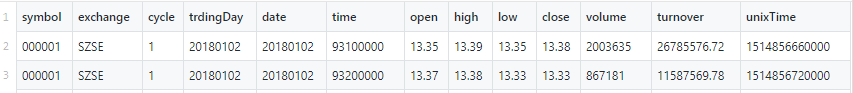
6.1. Partition Planning
First, we should plan how to partition the data. We need to determine the partitioning columns and the granularity of the partitions.
Columns that are frequently used in where, group by or context by clauses are good candidates for partitioning columns. As queries on stocks data often involve trading days and stock symbols, we recommend to use "tradingDay" column and "symbol" column to form a composite (COMPO) partition.
For optimal performance, each partition should have roughly the same size, and the size of each partition should be between 100MB and 1GB before compression. For details please refer to Partition Guidelines of DolphinDB Partitioned Database Tutorial.
We can use a range partition on the trading date (each year is a range), and a range partition on stock symbols (100 ranges) in the composite partition. In total we have 10*100=1000 partitions, and each partition has about 100MB data.
Use the following script to create the partition scheme for "tradingDay" column. It creates empty partitions for future data up to 2030.
yearRange =date(2008.01M + 12*0..22)Use the following script to create the partition scheme for "symbol" column. As each symbol has the same amount of data, we go through all annual directories to get a list of stock symbols, then use cutPoint function to divide them into 100 intervals. Considering that new stock symbols may be larger than the current maximum stock symbol, we add a stock symbol of 999999 as the maximum stock symbol.
// Traverse all the annual catalogs, to reorganize the stock code list, and divide into 100 intervals by cutPoint
symbols = array(SYMBOL, 0, 100)
yearDirs = files(rootDir)[`filename]
for(yearDir in yearDirs){
	path = rootDir + "/" + yearDir
	symbols.append!(files(path)[`filename].upper().strReplace(".CSV",""))
}
// Increase the expansion scope::
symbols = symbols.distinct().sort!().append!("999999");
// Divided into 100 parts
symRanges = symbols.cutPoints(100)
Create a partitioned database with a composite (COMPO) partition and a table "stockData" with the following script:
columns=`symbol`exchange`cycle`tradingDay`date`time`open`high`low`close`volume`turnover`unixTime
types =  [SYMBOL,SYMBOL,INT,DATE,DATE,TIME,DOUBLE,DOUBLE,DOUBLE,DOUBLE,LONG,DOUBLE,LONG]

dbDate=database("", RANGE, yearRange)
dbID=database("", RANGE, symRanges)
db = database(dbPath, COMPO, [dbDate, dbID])

pt=db.createPartitionedTable(table(1000000:0,columns,types), `stockData, `tradingDay`symbol);
6.2. Import Data
We import data by going through the directories to read and write all CSV files to the distributed table dfs://SAMPLE_TRDDB.
First, the data format of a column in a CSV file might be different from that in DolphinDB. For example, milliseconds in timestamps might be saved as integers in a CSV file. To convert them to milliseconds in timestamps in DolphinDB, we can use the temporal conversion function datetimeParse together with the formatting function format:
datetimeParse(format(time,"000000000"),"HHmmssSSS")It takes a long time to use a single-thread loop operation to import 100GB data. To fully utilize the cluster resources, we can divide the importing task into multiple subtasks to be executed on all nodes in parallel. Each subtask imports a year's data. This process is implemented in the following two steps:
First, define a function to import all data files in an annual directory:
def loadCsvFromYearPath(path, dbPath, tableName){
	symbols = files(path)[`filename]
	for(sym in symbols){
		filePath = path + "/" + sym
		t=loadText(filePath)
		database(dbPath).loadTable(tableName).append!(select symbol, exchange,cycle, tradingDay,date,datetimeParse(format(time,"000000000"),"HHmmssSSS"),open,high,low,close,volume,turnover,unixTime from t )
	}
}
Next, the function defined above is used with submitJob function and rpc function to submit the tasks to each node in the cluster to execute:
nodesAlias="NODE" + string(1..4)
years= files(rootDir)[`filename]

index = 0;
for(year in years){
	yearPath = rootDir + "/" + year
	des = "loadCsv_" + year
	rpc(nodesAlias[index%nodesAlias.size()],submitJob,des,des,loadCsvFromYearPath,yearPath,dbPath,`stockData)
	index=index+1
}
During the data importing process, we can monitor the status of the tasks with pnodeRun(getRecentJobs).
In DolphinDB, partitions are the smallest units to store data and writing access to a partition is exclusive. We should avoid writing to the same partition from multiple tasks at the same time. In the example above, each task writes a different year's data, so it is impossible to write to the same partition by multiple tasks at the same time.
The script for this example can be downloaded from the Appendix.