A Guide to SOCP: From Problem Formulation to Solution

In quantitative finance, optimization solvers are essential tools for tackling complex decision-making problems in portfolio optimization, risk assessment, and asset pricing. DolphinDB's suite of optimization solver functions - including linprog, quadprog, qclp, and socp - enables practitioners to translate financial problems into mathematical models and find optimal solutions.

Among these, the socp function (for second-order cone programming problems) is particularly effective for handling uncertainty and nonlinear constrains. In risk management, it efficiently handles quadratic constraints, such as those involving variance and standard deviation calculations. In portfolio optimization, it manages various market complexities, such as leverage limits, market exposure constraints, and capital requirements. Additionally, the socp function demonstrates superior computational efficiency when handling large datasets, allowing it to quickly converge to globally optimal solutions.

This article provides a comprehensive introduction to the socp function in DolphinDB, using a practical portfolio optimization example to demonstrate how real-world financial problems can be reformulated and solved with the SOCP problem.

1. Mathematical Model of SOCP Problems

The socp function is used to solve Second-Order Cone Programming (SOCP) problems, which are highly versatile and applicable in a wide range of scenarios. While DolphinDB provides specialized functions for specific optimization types like Linear Programming (LP), Quadratic Programming (QP), and Quadratically Constrained Linear Programming (QCLP), these problems can alternatively be solved using the socp function by reformulating them into SOCP format (see Section 3).

To better understand the socp function and how to transform optimization problems into SOCP form, we will first introduce the mathematical model of SOCP and explain which types of optimization problems it can address.

1.1 Cone Representation of SOCP Problems

where,

K is the cone.
s is a slack variable whose value is determined during optimization.
f is a numerical vector indicating the coefficient vector of the objective function.
G is a numerical matrix indicating the coefficient matrix of the cone constraints.
h is a numerical vector indicating the right-hand side of the cone constraints.
Aeq is a numerical matrix indicating the coefficient matrix of the equality constraints.
beq is a numerical vector indicating the right-hand side of the equality constraints.

The equation Gx+s=h encompasses all inequality constraints in an SOCP problem, including both linear inequalities and second-order cone constraints. The problem's dimensions are defined by two key parameters of the socp function: l and q. l is an integer that specifies the dimension of the non-negative orthant constraints, i.e., the dimension of the linear inequalities. q is a positive vector in the form [r0, r1,…, rN-1], which contains the dimensions for each second-order cone constraint. Note that each dimension in q should be incremented by 1, accounting for both the 2-norm term on the left-hand side and the scalar term on the right-hand side of the inequality. Thus, the total l+sum(q) should equal the number of rows in matrix G.

1.2 Standard form of SOCP Problems

The standard form of an SOCP problem can be transformed into the cone form described above, allowing us to determine the corresponding parameters G, h, l, and q of the socp function for solving the problem. Below, we explain how to derive the cone form from the standard form to provide a clearer understanding.

1.Refomulate the second-order cone constraints

2.Combine these constraints and introduce an auxiliary variable s

The resulting forms of G and h are as follows:

2. Converting Programming Problems to SOCP Form

The conversion of general programming problems to SOCP requires transforming the original problem into SOCP standard form by constructing appropriate parameters based on the relationship between cone representation and standard form.

2.1 SOCP Form of Linear Programming

A linear programming problem involves optimizing a linear objective function subject to linear constraints. Its form is as follows:

For problems with linear inequality constraints , we can rearrange terms for .

For the linear constraints of the variable x, upper and lower bounds can be converted to

Standard SOCP form:

Where E is an identity matrix of the same dimension as x.

Construct the parameters:

2.2 SOCP Form of Quadratic Inequality Constraints

A quadratically constrained linear problem involves optimizing a linear objective function subject to constraints that contain quadratic terms. Its form is as follows:

For quadratic inequality constraints where V is a positive definite matrix and k is a positive scalar. V can be decomposed using Cholesky decomposition into V = F^TF. The original constraint can then be transformed:

Standard SOCP form:

Construct the parameters:

Where n indicates the length of variable x.

2.3 SOCP Form of Absolute Value Constraints

An absolute value constrained problem involves optimizing a linear objective function subject to linear constraints, with some constraints containing absolute values. Its form is as follows:

The 1-norm constraints can be expressed as the absolute value constraints.

By introducing auxiliary variable u_i

We can rewrite the problem in terms of the vector [x^T, u₁, ··· , u_n]^T and convert it into the SOCP form.

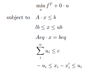
Construct the parameters:

2.4 SOCP Form of Quadratic Programming

A quadratic programming problem involves optimizing a quadratic objective function subject to linear constraints. Its form is as follows:

For such problems, we can introduce an auxiliary variable y = x^THx, where H is a positive definite matrix. Through Cholesky decomposition, H can be decomposed into H = U^TU. By applying the parallelogram identity, the problem can be transformed to:

Second-order cone constraints:

Standard SOCP form:

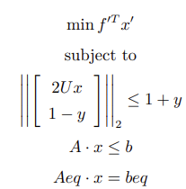
Where

Construct the parameters:

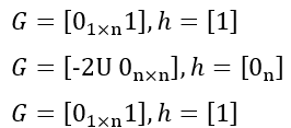
3. Use Cases

In this section, we will explore two portfolio optimization cases that illustrate how to reformulate financial problems into the SOCP format. Through these examples, we'll demonstrate step-by-step how to use the socp function to obtain optimal solutions.

3.1 Portfolio Optimization: with Linear Programming

This case demonstrates how to reformulate a linear stock portfolio optimization problem into SOCP format. The objective is to maximize expected returns while satisfying multiple weight constraints.

3.1.1 Mathematical Model

The problem can be transformed into a mathematical model with the objective function as follows:

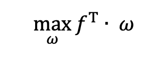
Where:

is target weight of each stock in the portfolio
is expected return of each stock in the portfolio

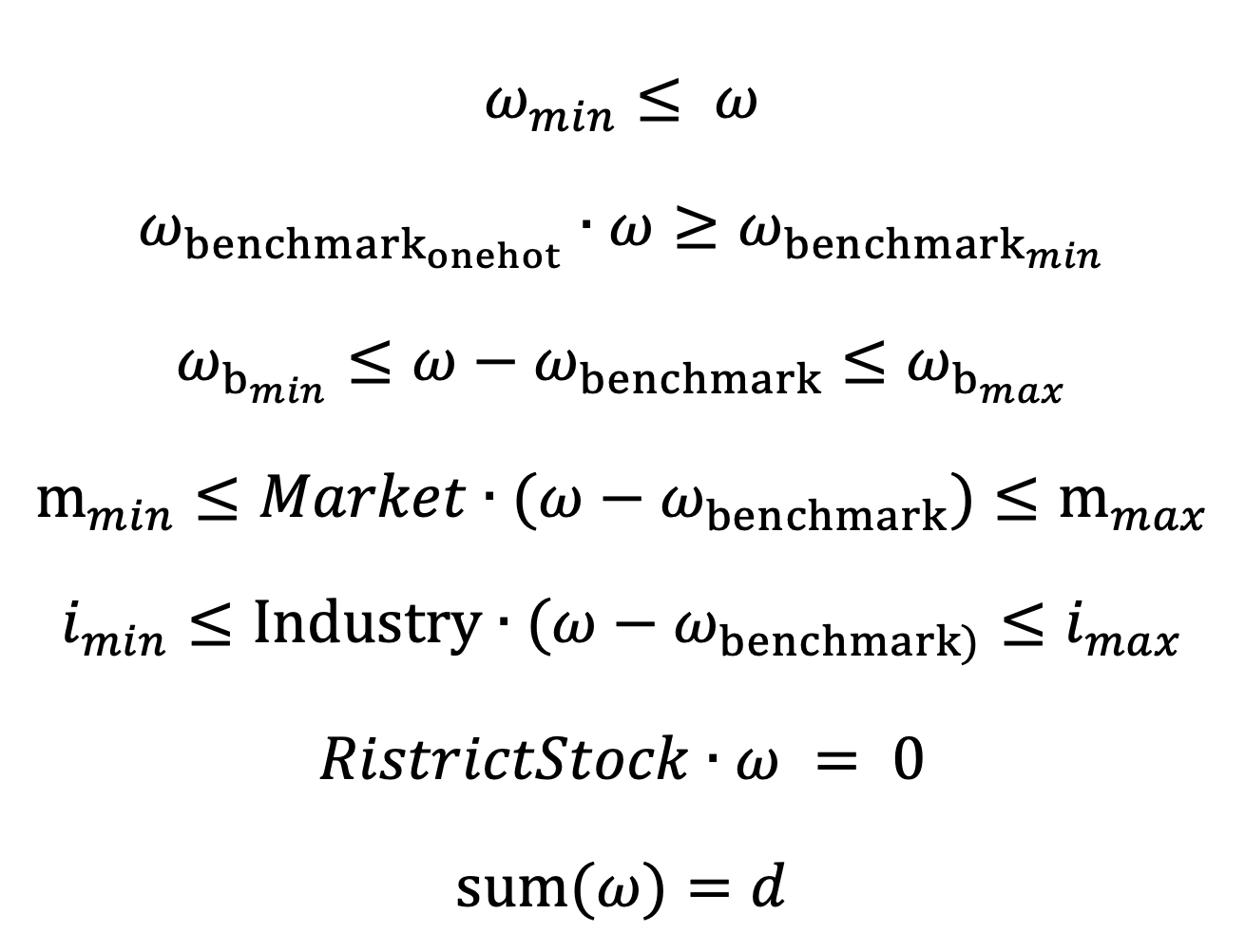
The model includes the following constraints for:

Individual stock weight
Component stock weight
Deviation for component stock weights
Market capitalization weight
Industry weight
Prohibition of investing in certain stocks
Target stock weights

Specifically:

Note: The first six constraints are linear inequalities that can be directly transformed by following the steps outlined in Section 2.1, while the seventh constraint involves equality conditions and must be defined using Aeq and beq.

3.1.2 Defining Parameters

The syntax of the socp function is socp(f, [G], [h], [l], [q], [A], [b]). Below are the steps to define the parameters.

Coefficient vector of the objective function (f): Since the socp function minimizes the objective function by default, negate the original expected returns:

f_1 = -f

Coefficient matrix for cone constraints (G):

unit_matrix = eye(vector_size)//vector_size is the number of stocks in portfolio
G = concatMatrix([-unit_matrix, -transpose(matrix(w_b_onehot))], false)  // individual stock weight and component stock weight
G = concatMatrix([G, unit_matrix], false)  // component stock deviation <max>
G = concatMatrix([G, -unit_matrix], false)  // component stock deviation <min>
G = concatMatrix([G, transpose(matrix(market_vector))], false)  // market capitalization weight <max>
G = concatMatrix([G, -transpose(matrix(market_vector))], false)  // market capitalization weight <min>
G = concatMatrix([G, transpose(matrix(industry_matrix))], false)  // industry weight <max>
G = concatMatrix([G, -transpose(matrix(industry_matrix))], false)  // industry weight <min>

Right-hand-side vector for cone constraints (h):

h = array(DOUBLE).append!(w_min)  // individual stock weight
h.append!(-w_b_t_min)  // component stock weight
cs_max_temp = w_b_max + w_b  // component stock deviation <max>
h.append!(cs_max_temp)
cs_min_temp = -w_b_min - w_b  // component stock deviation <min>
h.append!(cs_min_temp)
mk_max_temp = m_max + transpose(matrix(market_vector))**w_b // market capitalization weight <max>
h.append!(mk_max_temp[0])
mk_min_temp = -m_min - transpose(matrix(market_vector))**w_b  // market capitalization weight <min>
h.append!(mk_min_temp[0])
ind_max_temp = ind_max + transpose(matrix(industry_matrix))**w_b // industry weight <max>
h.append!(ind_max_temp[0])
ind_min_temp = -ind_min - transpose(matrix(industry_matrix))**w_b  // industry weight <min>
h.append!(ind_min_temp[0])

Dimension of non-negative orthant constraints (l): As all constraints are linear, l equals the size of h:

l = h.size()

Dimension size of second-order cone constraints (q): As there are no second-order cone constraints in this example, q is set to an empty vector.

q = []

Coefficient matrix and right-hand-side vector for equality constraints (Aeq and beq):

one_vector = matrix(DOUBLE, 1, vector_size, , 1)
Aeq = concatMatrix([one_vector, transpose(matrix(restrict_stock))], false)  // target stock weight and prohibited stock
beq = array(DOUBLE).append!(d) // target stock weight
beq.append!(0)  // prohibited stock

3.1.3 Solving the Optimization Problem

Invoke the socp function with the defined parameters:

res = socp(f_1, G, h, l, q, Aeq, beq)

3.2 Portfolio Optimization: with Turnover Constraints and Tracking Error Constraints

This case extends the MVO (Mean-Variance Optimization) model to optimize a portfolio by balancing return maximization and risk minimization. It introduces additional constraints, including turnover constraints (limit portfolio rebalancing costs) and tracking error constraints (limit the portfolio's volatility relative to the benchmark), alongside those from the previous example.

3.2.1 Mathematical Model

The problem can be transformed into a mathematical model with the objective function as follows:

Where:

∑ is covariance matrix of returns.
ω₀ is the last position, i.e., the weight of the last individual stock weight.
C^T is coefficient for turnover costs.
λ is coefficient for risk aversion.

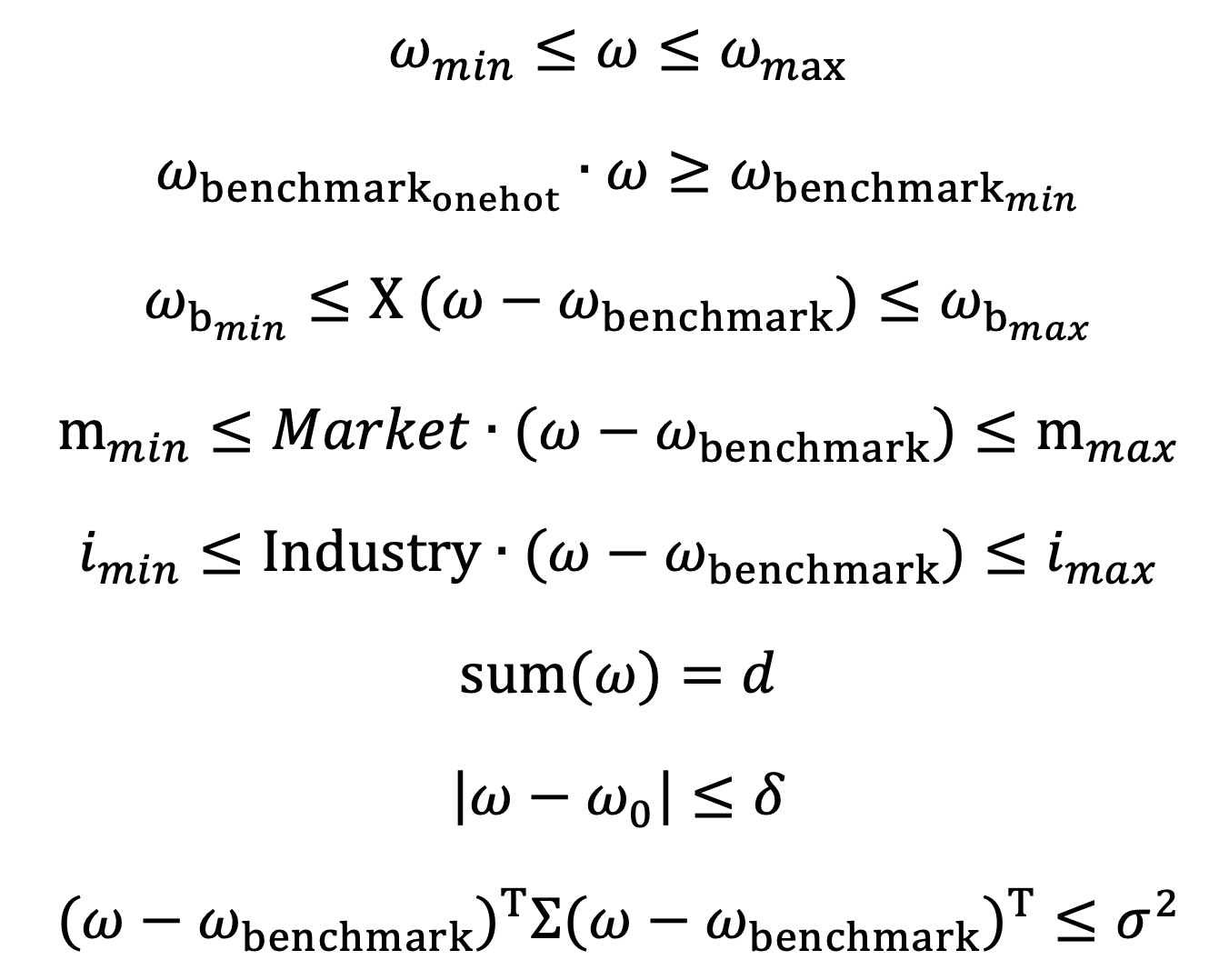
The constraints include:

Note: The first six constraints are linear constraints similar to those in the previous case. The seventh constraint, dealing with turnover, is a 1-norm (absolute value) constraint. The eighth constraint, which addresses tracking error, is a quadratic inequality constraint.

3.2.2 Reformulating Objective Function and Constraints

To solve this problem using SOCP, both the objective function and constraints need to be reformulated into an SOCP standard form.

Objective function

Introduce auxiliary variables for quadratic terms and for absolute value terms in turnover constraints. The objective function can be reformulated as follows:

Linear Constraints

The first six linear constraints are similar to those in the previous case and will not be repeated here.

Turnover Constraint

The turnover constraint, involving absolute values (1-norm), is reformulated using auxiliary variable u to fit SOCP format.

Tracking Error Constraint

The tracking error constraint is a quadratic inequality constraint that can be reformulated using the Cholesky decomposition:

Thus, the original constraint can be transformed into the following SOCP form (specific steps can be referenced in Section 2.2):

3.2.3 Defining Parameters

Below are the steps to define the parameters:

Coefficient vector of the objective function (f): New variables are introduced for the objective function.

// minimize f^T * w + 0 * u + lamda*y
c = f // coefficients for w 
c.append!(take(0, N)) // 0 * u
c.append!(take(lamda, 1)) // lamda*y

Coefficient matrix for cone constraints (G):

E = eye(N)// N refers to the number of w
zeros = matrix(DOUBLE, N, N, ,0)// auxiliary variables u
// linear inequality constraints
G = concatMatrix([E,zeros]) // w<=wmax
G = concatMatrix([G, concatMatrix([-E,zeros])], false) // -w <= -wmin
G = concatMatrix([G, concatMatrix([ -wb_one, matrix(DOUBLE,1,N,,0) ] ) ], false) // -w*wb_one <= -w_bmin 
G = concatMatrix([G, concatMatrix([ X, matrix(DOUBLE,1,N,,0) ])], false) // Xw <= xn+Xwb, deviation for component stock
G = concatMatrix([G, concatMatrix([-X, matrix(DOUBLE,1,N,,0)])], false) // -Xw <= -x1+Xwb
G = concatMatrix([G, concatMatrix([H, zeros ] ) ], false) // Hw <= hn+Hwb, market capitalization
G = concatMatrix([G, concatMatrix([-H, zeros ])], false) // -Hw <= -h1+Hwb
G = concatMatrix([G, concatMatrix([F, matrix(DOUBLE,1,N,,0)])], false) // F<= fn+Fwb, industry weight
G = concatMatrix([G, concatMatrix([-F, matrix(DOUBLE,1,N,,0)])], false) // -Fw <= -f1+wb
// turnover Constraint
G = concatMatrix([G, concatMatrix([ matrix(DOUBLE,1,N,,0), matrix(DOUBLE,1,N,,1) ] ) ], false) // sum( u_i ) <= delta
G = concatMatrix([G, concatMatrix([E,-E])], false) // w_i -u_i <= w`_i 
G = concatMatrix([G, concatMatrix([-E,-E])], false) // -w_i-u_i <= -w`_i
G = concatMatrix([G, concatMatrix([matrix(DOUBLE,1,N,,0), matrix(DOUBLE,1,N,,0)])], false)  // || Uw - Uwb ||2 <= delta   delta=0.5
G = concatMatrix([G, concatMatrix([-UT, Z]) ], false)  // UT is the covariance matrix after Cholesky decomposition
// add the coefficients for the auxiliary variable y
GZ = matrix(DOUBLE, G.shape()[0], 1, , 0) 
G = concatMatrix([G, GZ])
// the second-order cone coefficient matrix for the auxiliary variable y
GY = concatMatrix([ matrix(DOUBLE, 1, N, , 0) , matrix(DOUBLE, 1, N, , 0)   ])
G = concatMatrix([G, concatMatrix([GY, matrix([-1]) ] ) ], false)  // || [2Uw, -y] +[0 , 1]  ||2 <= y + 1   y
ZY = matrix(DOUBLE, U.shape()[0], N, , 0) 
GY = concatMatrix([2*U, ZY ])
G = concatMatrix([G, concatMatrix([GY, matrix(DOUBLE, U.shape()[0], 1, , 0)  ])], false)  // || [2Uw, -y] +[0 , 1]  ||2 <= y + 1   2U
GY = concatMatrix([matrix(DOUBLE,1,N,,0), matrix(DOUBLE,1,N,,0)])
G = concatMatrix([G, concatMatrix([GY, matrix([1])  ] ) ], false)  // || [2Uw, -y] +[0 , 1]  ||2 <= y + 1   -y

Right-hand-side vector for cone constraints (h) and dimension of non-negative orthant constraints (l):

// linear constrains
h = array(DOUBLE).append!(take(w_max, N)) // w<=w_max
h.append!(take(-wmin, N)) // -w <= -w_min
h.append!(-w_bmin) // -w*wb_one <= -w_bmin
temp = -X[N-1]+X**wb
h.append!(temp[0]) // Xw <= X[0]+X*wb
temp = -X[0]+X**wb
h.append!(-temp[0]) // -Xw <= xn+Xwb
temp = -H[,N-1]+H**wb
temp = exec * from table(temp)
h.append!( temp ) // Hw <= hn+Hwb
temp = -H[,0]+H**wb
temp = exec * from table(temp)
h.append!(-temp) //  -Hw <= -h1+Hwb
temp = -F[N-1]+F**wb
h.append!(temp[0]) // F<= fn+Fwb
temp = -F[0]+F**wb
h.append!(-temp[0]) //  -Fw <= -f1+wb
h.append!(delta) 
h.append!(w0) 
h.append!(-w0)
l = h.size() 
// quadratic constraints
h.append!(delta) 
temp = exec * from table(U**wb)
h.append!(temp)  
h.append!(take(1, 1)) //|| [2Uw, -y] +[0 , 1]  ||2 <= y + 1  
h.append!(take(0, N)) //|| [2Uw, -y] +[0 , 1]  ||2 <= y + 1  
h.append!(take(1, 1)) //|| [2Uw, -y] +[0 , 1]  ||2 <= y + 1

Dimension size of second-order cone constraints (q):

q = [ U.shape()[0]+1, U.shape()[0]+1+1 ]

Coefficient matrix and right-hand-side vector for equality constraints (Aeq and beq):

temp = concatMatrix([matrix(DOUBLE, 1, N, ,1), matrix(DOUBLE, 1, N, ,0)])
Aeq = concatMatrix([ temp , matrix(DOUBLE, 1, 1, ,0)])
beq = array(DOUBLE).append!(1)

3.2.4 Solving the Optimization Problem

Invoke the socp function with the defined parameters:

res = socp(c, G, h, l, q, Aeq, beq)

4. Summary

The socp function is the most commonly used optimization solver function in DolphinDB. Many complex convex optimization problems can be solved by reformulating them into SOCP form. Due to well-developed algorithmic solutions for SOCP, the function delivers superior computational performance, particularly when solving large-scale optimization problems.