Unified Stream and Batch Processing: Reactive State Engine
In high-frequency trading, we need to develop factors whose values are affected by each row of new data. These factors are stateful: not only are they affected by newest values of variables, they are also affected by past values of variables. Most people write Python programs to develop these high-frequency factors and then write C++ programs for real-time calculation in production. It is quite a heavy burden to develop 2 sets of code. Moreover, users needs to make sure the 2 sets of code produces the same result.
This tutorial introduces how to use the Reactive State Engine released by DolphinDB 1.30.3 to conduct both batch and stream calculation with the same set of code. The state engine accepts expressions or functions written in batch processing of historical data (development stage) as input for stream calculation and ensures that the results of stream calculations are completely consistent with those of batch calculations. This avoids the cost of rewriting development code for production and making sure the 2 sets of code deliver the same result.
1. An example of High-frequency Factor
This section uses an example to introduce the challenges of high-frequency factor calculation. The following script is written in DolphinDB and uses a user-defined function sum_diff and a built-in function ema (exponential moving average). For more detailes about ema, please refer to What is EMA? How to Use Exponential Moving Average With Formula. sum_diff is a stateless function, while ema is a stateful function which is affected by historical data. What makes the calculation even trickier is that, as shown in the diagram below, the calculation uses multiple levels of nested ema function.
def sum_diff(x, y){
    return (x-y)/(x+y)
}

ema(1000 * sum_diff(ema(price, 20), ema(price, 40)),10) -  ema(1000 * sum_diff(ema(price, 20), ema(price, 40)), 20)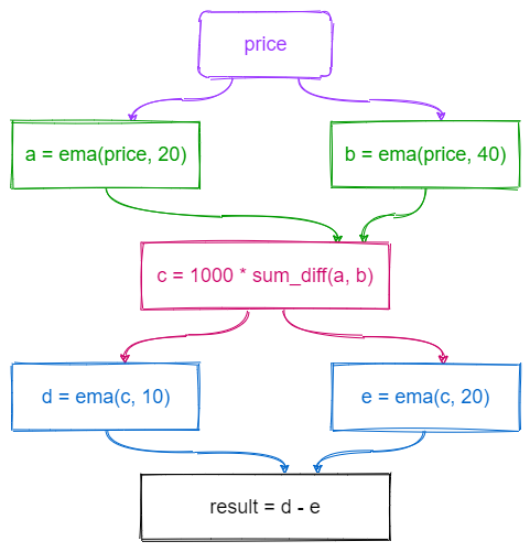
For scenarios like this, we need to solve the following problems:
- Can we quickly calculate 100~1000 factors for each stock with historical data during development stage?
- Can we calculate 100~1000 factors for each stock as soon as new tick data arrives in real-time trading?
- Are the codes for batch computing and for stream computing efficient? Can they be unified? Is it easy to check if they produce the same results?
2. Pros and Cons of Existing Solutions
Python pandas/numpy is currently the most commonly used solution for developing high-frequency factors. Pandas offers a comprehensive solution for panel data processing, and its built-in functions include most of the operators needed for high-frequency factor calculations. High-frequency factors can be developed quickly in pandas. However, pandas has poor performance in both historical data and real-time data calculation. With historical data, there is room for improvements in pandas' single-threaded calculations. Moreover, due to the limitation of Python's global interpreter lock, parallel calculations cannot be conducted in pandas. With real-time data, as Python does not support Incremental calculation, it cannot meet the performance requirements of real-time calculation.
In consideration of these performance issues of pandas, most organizations will rewrite the pandas code for development in C++ for production. This is very costly as two sets of code need to be maintained and a significant amount of effort would be spent to ensure that the results of the two sets of code are exactly the same.
Apache Flink takes a unified approach to batch and stream processing. Flink supports SQL and window functions. Commonly used operators for high-frequency factors have been implemented in Flink. Hence, simple factors can be calculated with Flink efficiently. Nonetheless, the biggest problem with Flink is that it cannot fulfill complex calculations. In the example mentioned in previous chapter, multiple levels of nested window functions is required, but it cannot be implemented directly with Flink. This is the motivation for DolphinDB to develop a reactive state engine.
3. Reactive State Engine
The reactive state engine is a black box. The inputs are real-time data and the functions or expressions for calculations with historical data, and the output is the factor value. Since developing and verifying high-frequency factors on historical data is much easier than on real-time data, the reactive state engine significantly reduces the development cost.
def sum_diff(x, y){
    return (x-y)/(x+y)
}
factor1 = <ema(1000 * sum_diff(ema(price, 20), ema(price, 40)),10) -  ema(1000 * sum_diff(ema(price, 20), ema(price, 40)), 20)>

share streamTable(1:0, `sym`price, [STRING,DOUBLE]) as tickStream
result = table(1000:0, `sym`factor1, [STRING,DOUBLE])
rse = createReactiveStateEngine(name="reactiveDemo", metrics =factor1, dummyTable=tickStream, outputTable=result, keyColumn="sym")
subscribeTable(tableName=`tickStream, actionName="factors", handler=tableInsert{rse})
The above code implements the streaming calculation of the aforementioned factor in DolphinDB. "factor1" is the code to calculate the aforementioned factor with historical data. It can be directly passed to the reactive state engine "rse" for streaming calculation. Through the function subscribeTable, the stream table "tickStream" is associated with the state engine "rse". Each batch of real-time data ingestion will trigger the calculation by the reactive state engine and the factor values are output to the table "result". The following code generates random data and injects it into the stream table "tickStream". The result is exactly the same as that from the SQL statement with historical data.
data = table(take("000001.SH", 100) as sym, rand(10.0, 100) as price)
tickStream.append!(data)
factor1Hist = select sym, ema(1000 * sum_diff(ema(price, 20), ema(price, 40)),10) -  ema(1000 * sum_diff(ema(price, 20), ema(price, 40)), 20) as factor1 from data context by sym
assert each(eqObj, result.values(), factor1Hist.values())
3.1. How it works
As shown in Figure 1, a stateful high-frequency factor calculation process can actually be decomposed into a directed acyclic graph (DAG). There are three kinds of nodes in the graph: (1) data sources, such as price, (2) stateful operators, such as a, b, d, e (3) stateless operators, such as c and result. Starting from the data source node, following the established path, layer by layer, we can get the final factor output. This process is remarkably similar to calculation chain in excel. When the data of a cell changes, the associated cells change sequentially. The name of the ReactiveStateEngine is also derived from this point.
Stateless operators are relatively simple and could be expressed and calculated using DolphinDB's existing script engine. Consequently, the problem can be transformed into two points: (1) how to parse an optimal DAG, (2) how to optimize the calculation of each stateful operator.
3.2. Strength
DolphinDB's scripting language is a multi-paradigm programming language that supports vector programming and functional programming. Through function call relation, it is not difficult to get the DAG of the calculation steps. When parsing, because the schema of the input message is known, we can quickly infer the data type of input and output from each node. After the input parameter type and the function name is determined, the specific instance of each state operator can be created.
Each operator (stateful and stateless) can be transformed into a unique string sequence in DolphinDB. Based on this, we can delete duplicate operators and improve computational efficiency.
3.3. Built-in State Function
The state operator needs to use the historical state when calculating. If every calculation needs to use all historical data to do full calculation, it will not only consume memory, but also consume CPU time. The optimization of the state function, that is, the streaming implementation of incremental computing, is overly critical. The following state functions have been optimized and implemented in DolphinDB's ReactiveStateEngine. Currently, the state engine does not allow to use unoptimized state functions.
- Cumulative window function: cumavg, cumsum, cumprod, cumcount, cummin, cummax, cumvar, cumvarp, cumstd, cumstdp, cumcorr, cumcovar, cumbeta, cumwsum, cumwavg
- Moving window function: ema, mavg, msum, mcount, mprod, mvar, mvarp, mstd, mstdp, mskew, mkurtosis, mmin, mmax, mimin, mimax, mimaxLast, miminLast, mmed, mpercentile, mrank, mcorr, mcovar, mbeta, mwsum, mwavg, mslr
- Sequence correlation function: deltas, ratios, ffill, move, prev, iterate, ewmMean, ewmVar, ewmStd, ewmCovar, ewmCorr
Except for mslr that returns two values, the rest above functions have only one return value. In future release, DolphinDB will allow users to use plug-ins to develop their own state functions, which can be used in the state engine.
3.4. User-defined State Function
User-defined functions can be used in ReactiveStateEngine. Following points need to be noticed:
- Use @state to declare that the function is a user-defined state function before definition.
- Only assignment statements and return statements can be used in user-defined state functions. The return statement can return multiple values and must be the last statement.
- Use "iif" function to represent the logic of if...else.
If only one expression is allowed to represent a factor, it will bring many limitations. First, in some cases, a factor cannot be completely realized using only expressions. The following example returns alpha, beta and residual in linear regression.
@state
def slr(y, x){
    alpha, beta = mslr(y, x, 12)
    residual = mavg(y, 12) - beta * mavg(x, 12) - alpha
    return alpha, beta, residual
}
Secondly, many factors may use common intermediate results. When multiple factors are defined, the code will be more concise. User-defined functions can return multiple results at the same time. The following function multiFactors defines 5 factors.
@state
def multiFactors(lowPrice, highPrice, volumeTrade, closePrice, buy_active, sell_active, tradePrice, askPrice1, bidPrice1, askPrice10, agg_vol, agg_amt){
    a = ema(askPrice10, 30)
    term0 = ema((lowPrice - a) / (ema(highPrice, 30) - a), 50)
    term1 = mrank((highPrice - a) / (ema(highPrice, 5) - a), true,  15)
    term2 = mcorr(askPrice10, volumeTrade, 10) * mrank(mstd(closePrice, 20, 20), true, 10)
    buy_vol_ma = mavg(buy_active, 6)
    sell_vol_ma = mavg(sell_active, 6)
    zero_free_vol = iif(agg_vol==0, 1, agg_vol)
    stl_prc = ffill(agg_amt \ zero_free_vol \ 20).nullFill(tradePrice)
    buy_prop = stl_prc

    spd = askPrice1 - bidPrice1
    spd_ma = round(mavg(iif(spd < 0, 0, spd), 6), 5)
    term3 = buy_prop * spd_ma
    term4 = iif(spd_ma == 0, 0, buy_prop / spd_ma)
    return term0, term1, term2, term3, term4
}
Finally, some expressions are verbose and lack readability. Changing the factor expression in the first section to user-defined function factor1 below, the calculation logic is clearer.
@state
def factor1(price) {
    a = ema(price, 20)
    b = ema(price, 40)
    c = 1000 * sum_diff(a, b)
    return  ema(c, 10) - ema(c, 20)
}
3.5. Output Filtering
The state engine will make a calculation response to each input message and produce a record as a result. The results will be output to the result table by default, which means that, inputting n messages will output n records. If you want your output only a part of the results, you could enable filter conditions, and only the results that meet the conditions will be output.
The following example checks whether the stock price has changed, and only the record of the price change will be output.
share streamTable(1:0, `sym`price, [STRING,DOUBLE]) as tickStream
result = table(1000:0, `sym`price, [STRING,DOUBLE])
rse = createReactiveStateEngine(name="reactiveFilter", metrics =[<price>], dummyTable=tickStream, outputTable=result, keyColumn="sym", filter=<prev(price) != price>)
subscribeTable(tableName=`tickStream, actionName="filter", handler=tableInsert{rse})
3.6. State Snapshot
In order to meet the needs of business continuity in the production environment, DolphinDB's built-in streaming engines, including ReactiveStateEngine, support snapshot output.
The snapshot of ReactiveStateEngine includes the ID of the last processed message and the current state of the engine. When an exception occurs in the system and the state engine is reinitialized, the engine can recover to the state of the last snapshot and will subscribe right from the next message.
def sum_diff(x, y){
    return (x-y)/(x+y)
}
factor1 = <ema(1000 * sum_diff(ema(price, 20), ema(price, 40)),10) -  ema(1000 * sum_diff(ema(price, 20), ema(price, 40)), 20)>

share streamTable(1:0, `sym`price, [STRING,DOUBLE]) as tickStream
result = table(1000:0, `sym`factor1, [STRING,DOUBLE])
rse = createReactiveStateEngine(name="reactiveDemo", metrics =factor1, dummyTable=tickStream, outputTable=result, keyColumn="sym", snapshotDir= "/home/data/snapshot", snapshotIntervalInMsgCount=400000)
msgId = getSnapshotMsgId(rse)
if(msgId >= 0) msgId += 1
subscribeTable(tableName=`tickStream, actionName="factors", offset=msgId, handler=appendMsg{rse}, handlerNeedMsgId=true)
To enable the snapshot for ReactiveStateEngine, you need to specify two additional parameters "snapshotDir" and "snapshotIntervalInMsgCount". "snapshotDir" is used to specify the directory where the snapshot is stored. "snapshotIntervalInMsgCount" specifies how many messages are processed to generate a snapshot. When the engine is initialized, the system will check whether there is a file named by the engine and saved with an extension .snapshot. Take the above code as an example, if the file /home/data/snapshot/reactiveDemo.snapshot exists, it will load the snapshot. The function getSnapshotMsgId can get the most recent msgId of the snapshot. If there is no snapshot, it will return -1.
To enable the snapshot in state engine, the subscribeTable function also needs to be modified accordingly:
- First, the offset of the message must be specified.
- Secondly, the handler must use the
appendMsgfunction. TheappendMsgfunction accepts two parameters,msgBodyandmsgId. - Finally, the parameter
handlerNeedMsgIdmust be set as true.
3.7. Parallel Computing
When a large number of messages need to be processed, the optional parameters "filter" and "hash" shall be specified in DolphinDB's subscribeTable Function to allow multiple subscription clients to process messages in parallel. The logic is shown in the diagram below.
- The parameter "
filter" is used to specify message filtering logic. Currently, the filter parameter can be specified in the following 3 ways: value filtering, range filtering and hash filtering. - The parameter "
hash" can specify a hash value indicating which subscription executor will process the incoming messages for this subscription. For example, if the configuration parametersubExecutors=4 and the user specifies ahashvalue of 5, the calculation task will be processed by the second executor.
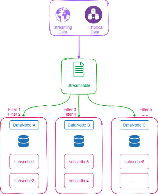
The following is an example of factors parallel computation using reactive state engine. Assuming that the configuration parameter subExecutors=4, and we create 4 state engines. Each state engine subscribes to different stock data according to the hash value of the stock code from streaming table, specifies different subscription executors for processing, and finally outputs the results to a same Output table.
def sum_diff(x, y){
    return (x-y)/(x+y)
}
factor1 = <ema(1000 * sum_diff(ema(price, 20), ema(price, 40)),10) -  ema(1000 * sum_diff(ema(price, 20), ema(price, 40)), 20)>

share streamTable(1:0, `sym`price, [STRING,DOUBLE]) as tickStream
setStreamTableFilterColumn(tickStream, `sym)
share streamTable(1000:0, `sym`factor1, [STRING,DOUBLE]) as resultStream

for(i in 0..3){
    rse = createReactiveStateEngine(name="reactiveDemo"+string(i), metrics =factor1, dummyTable=tickStream, outputTable=resultStream, keyColumn="sym")
    subscribeTable(tableName=`tickStream, actionName="sub"+string(i), handler=tableInsert{rse}, msgAsTable = true, hash = i, filter = (4,i))
}

n=2000000
tmp = table(take("A"+string(1..4000), n) as sym, rand(10.0, n) as price)
tickStream.append!(tmp)
Note that if multiple state engines use a same output table, the output table must be a shared table. Tables that are not shared are not thread-safe, and parallel writing may cause the system to crash.
4. Unified Stream and Batch Processing
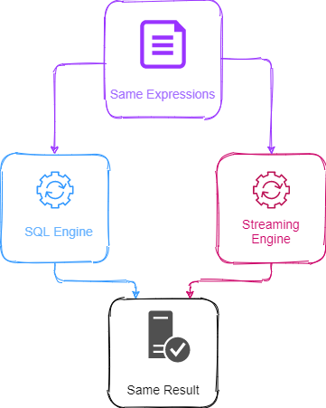
There are two ways to implement the unified stream and batch processing of high-frequency factors in DolphinDB.
The first method is to use functions or expressions to realize high-frequency factors, substituting them into different calculation engines to calculate based on historical data or streaming data. Substituting into SQL engine can realize the calculation of historical data; substituting into ReactiveStateEngine can realize the calculation of streaming data. This has been exemplified in the preamble of Chapter 3. In this mode, the expression in the DolphinDB is actually a factor's semantics description, rather than a specific implementation. The specific calculation is completed by the corresponding calculation engine, so as to achieve the best performance in different scenarios.
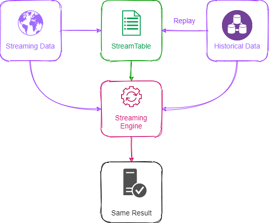
The second method is to use replay function to convert historical data into streaming data and then complete the calculation through streaming calculation engine. We still take the factor at the beginning of the tutorial as an example. The only difference is that the data source of the stream data "tickStream" comes from the replay of the historical database. Using this method to calculate factor based on historical data is not efficient.
def sum_diff(x, y){
    return (x-y)/(x+y)
}
factor1 = <ema(1000 * sum_diff(ema(price, 20), ema(price, 40)),10) -  ema(1000 * sum_diff(ema(price, 20), ema(price, 40)), 20)>

share streamTable(1:0, `sym`date`time`price, [STRING,DATE,TIME,DOUBLE]) as tickStream
result = table(1000:0, `sym`factor1, [STRING,DOUBLE])
rse = createReactiveStateEngine(name="reactiveDemo", metrics =factor1, dummyTable=tickStream, outputTable=result, keyColumn="sym")
subscribeTable(tableName=`tickStream, actionName="factors", handler=tableInsert{rse})

//Load one day's data from "trade" in historical database "dfs://TAQ" and replay it to stream table "tickStream".
inputDS = replayDS(<select sym, date, time, price from loadTable("dfs://TAQ", "trades") where date=2021.03.08>, `date, `time, 08:00:00.000 + (1..10) * 3600000)
replay(inputDS, tickStream, `date, `time, 1000, true, 2)
5. Performance Test
We tested the calculation performance of ReactiveStateEngine. The test uses simulated data and also uses warmupStreamEngine function to simulate the situation where the state engine has processed part of the data. The test includes a total of 20 factors in different complexity, of which two user-defined state functions return 3 and 5 factors respectively. To facilitate testing, the calculation uses only single-threaded processing.
@state
def slr(y, x){
    alpha, beta = mslr(y, x, 12)
    residual = mavg(y, 12) - beta * mavg(x, 12) - alpha
    return alpha, beta, residual
}

@state
def multiFactors(lowPrice, highPrice, volumeTrade, closePrice, buy_active, sell_active, tradePrice, askPrice1, bidPrice1, askPrice10, agg_vol, agg_amt){
    a = ema(askPrice10, 30)
    term0 = ema((lowPrice - a) / (ema(highPrice, 30) - a), 50)
    term1 = mrank((highPrice - a) / (ema(highPrice, 5) - a), true,  15)
    term2 = mcorr(askPrice10, volumeTrade, 10) * mrank(mstd(closePrice, 20, 20), true, 10)
    buy_vol_ma = mavg(buy_active, 6)
    sell_vol_ma = mavg(sell_active, 6)
    zero_free_vol = iif(agg_vol==0, 1, agg_vol)
    stl_prc = ffill(agg_amt \ zero_free_vol \ 20).nullFill(tradePrice)
    buy_prop = stl_prc

    spd = askPrice1 - bidPrice1
    spd_ma = round(mavg(iif(spd < 0, 0, spd), 6), 5)
    term3 = buy_prop * spd_ma
    term4 = iif(spd_ma == 0, 0, buy_prop / spd_ma)
    return term0, term1, term2, term3, term4
}

metrics = array(ANY, 14)
metrics[0] = <ema(1000 * sum_diff(ema(close, 20), ema(close, 40)),10) -  ema(1000 * sum_diff(ema(close, 20), ema(close, 40)), 20)>
metrics[1] = <mslr(high, volume, 8)[1]>
metrics[2] = <mcorr(low, high, 11)>
metrics[3] = <mstdp(low, 15)>
metrics[4] = <mbeta(high, value, 63)>
metrics[5] = <mcovar(low, value, 71)>
metrics[6] = <(close/mavg(close, 1..6)-1)*100>
metrics[7] = <mmin(high, 15)>
metrics[8] = <mavg(((high+low)/2+(mavg(high, 2)+mavg(low, 2))/2)*(high-low)/volume, 7, 2)>
metrics[9] = <mslr(mavg(close, 14), volume, 63)[1]>
metrics[10] = <mcorr(mavg(open, 25), volume, 71)>
metrics[11] = <mbeta(high, mstdp(close, 8), 77)>
metrics[12] = <slr(close, volume)>
metrics[13] = <multiFactors(low, high, volume, close, numTrade, numTrade, close, value, close, open, volume, numTrade)>

dummy = streamTable(10000:0, `symbol`market`date`time`quote_type`preclose`open`high`low`close`numTrade`volume`value`position`recvtime,[SYMBOL,SHORT,DATE,TIME,SHORT,DOUBLE,DOUBLE,DOUBLE,DOUBLE,DOUBLE,DOUBLE,LONG,DOUBLE,LONG,TIMESTAMP])

def prepareData(tickNum, batch){
    total = tickNum*batch
    data=table(total:total, `symbol`market`date`time`quote_type`preclose`open`high`low`close`numTrade`volume`value`position`recvtime,[SYMBOL,SHORT,DATE,TIME,SHORT,DOUBLE,DOUBLE,DOUBLE,DOUBLE,DOUBLE,DOUBLE,LONG,DOUBLE,LONG,TIMESTAMP])
    data[`market]=rand(10, total)
    data[`date]=take(date(now()), total)
    data[`time]=take(time(now()), total)
    data[`symbol]=take("A"+string(1..tickNum), total)
    data[`open]=rand(100.0, total)
    data[`high]=rand(100.0, total)
    data[`low]=rand(100.0, total)
    data[`close]=rand(100.0, total)
    data[`numTrade]=rand(100, total)
    data[`volume]=rand(100, total)
    data[`value]=rand(100.0, total)
    data[`recvtime]=take(now(), total)
    return data
}

dropStreamEngine("demo1")
dropStreamEngine("demo2")
dropStreamEngine("demo3")
dropStreamEngine("demo4")

//4000 stocks, 20 factors
hisData = prepareData(4000, 100)
realData = prepareData(4000, 1)
colNames = ["symbol"].append!("factor"+string(0..19))
colTypes = [SYMBOL].append!(take(DOUBLE, 20))
resultTable = streamTable(10000:0, colNames, colTypes)
engine1 = createReactiveStateEngine(name="demo1", metrics=metrics, dummyTable=dummy, outputTable=resultTable, keyColumn="symbol")
warmupStreamEngine(engine1, hisData)
timer(10) engine1.append!(realData)
dropAggregator("demo1")

//1 stock, 20 factors
hisData = prepareData(1, 100)
realData = prepareData(1, 1)
colNames = ["symbol"].append!("factor"+string(0..19))
colTypes = [SYMBOL].append!(take(DOUBLE, 20))
resultTable = streamTable(10000:0, colNames, colTypes)
engine2 = createReactiveStateEngine(name="demo2", metrics=metrics, dummyTable=dummy, outputTable=resultTable, keyColumn="symbol")
warmupStreamEngine(engine2, hisData)
timer(10) engine2.append!(realData)
dropAggregator("demo2")

//4000 stocks, 1 factor
hisData = prepareData(4000, 100)
realData = prepareData(4000, 1)
metrics3 = metrics[0]
colNames = ["symbol", "factor0"]
colTypes = [SYMBOL, DOUBLE]
resultTable = streamTable(10000:0, colNames, colTypes)
engine3 = createReactiveStateEngine(name="demo3", metrics=metrics3, dummyTable=dummy, outputTable=resultTable, keyColumn="symbol")
warmupStreamEngine(engine3, hisData)
timer(10) engine3.append!(realData)

//200 stocks, 20 factors
hisData = prepareData(200, 100)
realData = prepareData(200, 1)
colNames = ["symbol"].append!("factor"+string(0..19))
colTypes = [SYMBOL].append!(take(DOUBLE, 20))
resultTable = streamTable(10000:0, colNames, colTypes)
engine4 = createReactiveStateEngine(name="demo4", metrics=metrics, dummyTable=dummy, outputTable=resultTable, keyColumn="symbol")
warmupStreamEngine(engine4, hisData)
timer(10) engine4.append!(realData)
We counted the total time spent for 10 times and took the average as the single time spent. The server CPU used in the test is Intel(R) Xeon(R) Silver 4216 CPU @ 2.10GHz. In the case of single thread, the test results are as follows:
| Number of Stocks | Number of Factors | Elapsed Time(ms) |
|---|---|---|
| 4000 | 20 | 6 |
| 1 | 20 | 0.07 |
| 4000 | 1 | 0.8 |
| 200 | 20 | 0.2 |
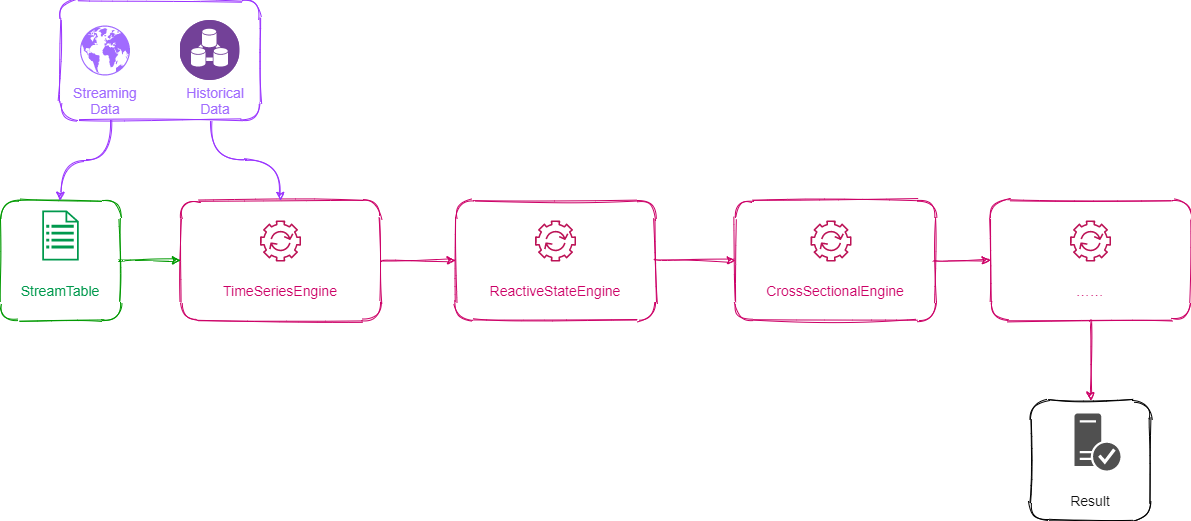
6. Streaming Engine Pipeline
The built-in streaming engine of DolphinDB includes ReactiveStateEngine, TimeSeriesEngine, CrossSectionalEngine, and AnomalyDetectionEngine. These engines all implement the data table (table) interface, so the pipeline processing of multiple engines becomes extremely simple, as long as the latter engine is used as the output of the previous engine. The process can be understood through the figure below. The pipeline processing can solve more complicated calculation problems. For example, factor calculation often requires using panel data to do a two-dimensional calculation of time series and cross section, which can be completed by connecting ReactiveStateEngine and CrossSectionalEngine in series.
The following example is a streaming realization of the No.1 factor from World Quant 101 quant factors. The rank function is a cross-sectional operation. The parameters of rank function are implemented with ReactiveStateEngine. The rank function itself is implemented with CrossSectionalEngine. The CrossSectionalEngine serves as the output of the ReactiveStateEngine.
Alpha#001: rank(Ts_ArgMax(SignedPower((returns<0?stddev(returns,20):close), 2), 5))-0.5

//create cross-sectional engine and calculate rank of each stock
dummy = table(1:0, `sym`time`maxIndex, [SYMBOL, TIMESTAMP, DOUBLE])
resultTable = streamTable(10000:0, `time`sym`factor1, [TIMESTAMP, SYMBOL, DOUBLE])
ccsRank = createCrossSectionalAggregator(name="alpha1CCS", metrics=<[sym, rank(maxIndex)\count(maxIndex) - 0.5]>,  dummyTable=dummy, outputTable=resultTable,  keyColumn=`sym, triggeringPattern='keyCount', triggeringInterval=3000, useSystemTime=false, timeColumn=`time)

@state
def wqAlpha1TS(close){
    ret = ratios(close) - 1
    v = iif(ret < 0, mstd(ret, 20), close)
    return mimax(signum(v)*v*v, 5)
}

//create reactive state engine and output to the cross-sectional engine 'ccsRank'
input = table(1:0, `sym`time`close, [SYMBOL, TIMESTAMP, DOUBLE])
rse = createReactiveStateEngine(name="alpha1", metrics=<[time, wqAlpha1TS(close)]>, dummyTable=input, outputTable=ccsRank, keyColumn="sym")
In the above example, we still need to manually distinguish which part is a cross-section operation and which part is a time series operation. In the future versions, DolphinDB will use row functions (rowRank, rowSum, etc.) to represent the semantics of cross-sectional operations, and other vector functions to represent time series operations, so that the system can automatically identify cross-sectional operations and time series operations in a factor expression, and further Automatically build an engine pipeline.
There is a big efficiency difference between pipeline processing and cascade processing of multiple streaming tables, though both can accomplish the same task. The latter involves multiple streaming data tables and multiple subscriptions, while the former only subscribed once, and all calculations are completed sequentially in one thread. Therefore, pipeline processing has better performance.
7. Future Work
ReactiveStateEngine has many commonly used built-in state operators, supports user-defined state functions, and can also be combined with other stream computing engines in a pipeline processing, which is convenient for developers to quickly implement complex high-frequency factors. In the future versions, the interface will be opened to allow users to develop state functions with C++ plug-ins to meet the needs of customization.
The built-in state operators are all developed in C++, and the algorithm has been optimized to achieve stream calculation of state operators in an incremental way, resulting in a particularly good performance when calculating on a single thread. For larger-scale tasks, you can split into multiple sub-subscriptions through subscription and filtering. Multiple nodes with multiple CPUs can complete the subscription calculation in parallel. Future Releases will improve the creation, management and monitoring functions of calculation sub-jobs, and change from manual to automatic.