Python Parser: Quantitative Analysis Quick Start
This tutorial is for: Python programmers learning to use DolphinDB
This tutorial covers:
- End-to-end factor development in DolphinDB using Python, including writing factor expressions and saving results
- Best practices for creating DolphinDB tables and databases via Python to store factors at various frequencies
- Sample Python code executable in DolphinDB for common factors
The DolphinDB Python Parser (referred to as the "Python Parser" in this tutorial) allows users to write and run Python code on the DolphinDB Server. It currently supports core Python syntax while incorporating some DolphinDB-specific extensions. With the Python Parser, you can write Python scripts in DolphinDB IDEs and submit them to the DolphinDB Server for execution. Since the Python Parser does not have the Global Interpreter Lock (GIL) constraint, it enables parallel computing. The Python syntax compatibility of Python Parser simplifies the learning curve for Python programmers new to DolphinDB.
1. Daily Factor Development from Tick Data: An End-to-End Example
This section demonstrates the overall workflow of factor development in DolphinDB using the Python Parser. The factor for calculating the percentage of closing auction volume on the day is used as an example.
1.1. Importing Historical Data
Before we can develop factors using the Python Parser, the market data must be imported into DolphinDB, including the OHLC prices at daily/minute frequencies, tick data, level 1 and level 2 snapshot data, etc.
For details on how to import data into DolphinDB, refer to DolphinDB tutorial: Importing text files or the user manual.
Since the data importing scripts provided in the aforementioned documentations is written in the DolphinDB scripting language, they must be executed using the DolphinDB interpreter. Based on which IDE you use, the steps to select the interpreter are different:
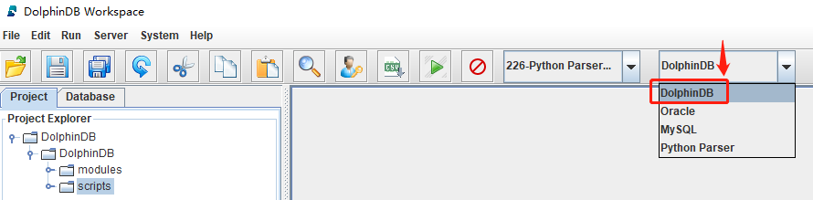
- DolphinDB GUI (get the latest version)
(1) Enable the language dropdown in the menu bar by clicking File > Preferences and check Always show language dropdown.
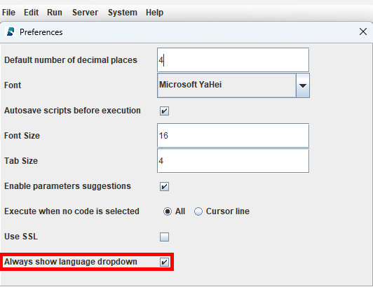
(2) In the menu bar, select DolphinDB from the language dropdown.
- Visual Studio Code (VS Code) with the DolphinDB extension (this tutorial uses V2.0.1041; get the latest version)
(1) In the VS Code, go to Manage > Settings, and search “@ext:dolphindb.dolphindb-vscode connections“.
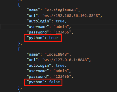
(2) Click Edit in settings.json to open the configuration file.
(3) In the dolphindb.connections list, each connection has a python attribute. Setting it to true means using the Python Parser interpreter. In this case, set it to “false“ to switch to the DolphinDB interpreter.
Execute the following script to import sample tick-by-tick trade data to DolphinDB, so you can run the example in this section.
Note: Before executing the script, first save the test data tradeData.csv (see Appendices) on your DolphinDB Server. Then replace the value of csvDir with the actual directory.
def createTB():
    dbName, tbName = "dfs://TL_Level2", "trade"
    # If a database with the same name already exists, delete it
    if existsDatabase(dbName):
        dropDatabase(dbName)
    # create a database with composite partitions -  VALUE partitioned by date and HASH partitioned by security ID
    db1 = database("", ddb.VALUE, seq(2020.01.01, 2021.01.01))
    db2 = database("", ddb.HASH, [ddb.SYMBOL, 50].toddb())
    db = database(dbName, ddb.COMPO, [db1, db2].toddb(), engine="TSDB")
    schemaTB = table(array(ddb.INT, 0) as ChannelNo,
                    array(ddb.LONG, 0) as ApplSeqNum,
                    array(ddb.SYMBOL, 0) as MDStreamID,
                    array(ddb.LONG, 0) as BidApplSeqNum,
                    array(ddb.LONG, 0) as OfferApplSeqNum,
                    array(ddb.SYMBOL, 0) as SecurityID,
                    array(ddb.SYMBOL, 0) as SecurityIDSource,
                    array(ddb.DOUBLE, 0) as TradePrice,
                    array(ddb.LONG, 0) as TradeQty,
                    array(ddb.SYMBOL, 0) as ExecType,
                    array(ddb.TIMESTAMP, 0) as TradeTime,
                    array(ddb.TIME, 0) as LocalTime,
                    array(ddb.LONG, 0) as SeqNo,
                    array(ddb.INT, 0) as DataStatus,
                    array(ddb.DOUBLE, 0) as TradeMoney,
                    array(ddb.SYMBOL, 0) as TradeBSFlag,
                    array(ddb.LONG, 0) as BizIndex,
                    array(ddb.SYMBOL, 0) as OrderKind,
                    array(ddb.SYMBOL, 0) as Market)
    db.createPartitionedTable(schemaTB, tbName, partitionColumns=["TradeTime", "SecurityID"].toddb(), compressMethods={"TradeTime":"delta"}.toddb(), sortColumns=["SecurityID", "TradeTime"].toddb(), keepDuplicates=ddb.ALL)

def loadData(csvDir):
    # create the database and table for tick-by-tick trade data
    createTB()

    # import test data from file
    name = ["ChannelNo", "ApplSeqNum", "MDStreamID", "BidApplSeqNum", "OfferApplSeqNum", "SecurityID", "SecurityIDSource", "TradePrice", "TradeQty", "ExecType", "TradeTime", "LocalTime", "SeqNo", "DataStatus", "TradeMoney", "TradeBSFlag", "BizIndex", "OrderKind", "Market"].toddb()
    type = ["INT", "LONG", "SYMBOL", "LONG", "LONG", "SYMBOL", "SYMBOL", "DOUBLE", "LONG", "SYMBOL", "TIMESTAMP", "TIME", "LONG", "INT", "DOUBLE", "SYMBOL", "LONG", "SYMBOL", "SYMBOL"].toddb()
    t = loadText(csvDir, schema=table(name, type))

    # append! data to database
    loadTable("dfs://TL_Level2", "trade").append!(t)

    # count the number of imported rows
    rowCount = select count(*) from loadTable("dfs://TL_Level2", "trade")      #	181,683
    print(rowCount)

# replace the value of csvDir with the actual directory on the DolphinDB server
csvDir = "/home/v2/downloads/data/tradeData.csv"
loadData(csvDir)
Note
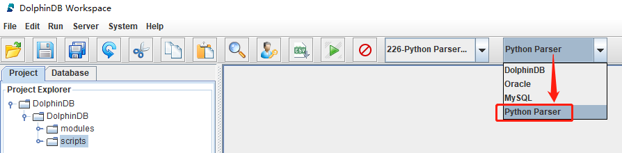
The example scripts provided in the rest of the tutorial are all written in Python and must be executed using the Python Parser interpreter. Refer to the steps above to switch interpreter in your IDE.
The screenshot below shows the GUI example.
1.2. Creating Database and Table
The following script creates the database and table for factors which analyze market data on a daily basis (referred to as "daily factors" for short) based on the DolphinDB best practices.
import pandas as pd
import dolphindb as ddb

dbName, tbName = "dfs://dayFactorDB", "dayFactorTB"

# If a database with the same name already exists, delete it
if existsDatabase(dbName):
    dropDatabase(dbName)

# create a database composite partitioned by year and factor name
db1 = database("", ddb.RANGE, date(datetimeAdd(1980.01M,seq(0,80)*12,'M')))
db2 = database("", ddb.VALUE, ["f1","f2"].toddb())
db = database(dbName, ddb.COMPO, [db1, db2].toddb(), engine='TSDB', atomic='CHUNK')

# create partitioned table
schemaTB = table(array(ddb.DATE, 0) as tradetime,
                array(ddb.SYMBOL, 0) as securityid,
                array(ddb.SYMBOL, 0) as factorname,
                array(ddb.DOUBLE, 0) as value)

db.createPartitionedTable(schemaTB, tbName, partitionColumns=["tradetime", "factorname"].toddb(), compressMethods={"tradetime":"delta"}.toddb(),
                        sortColumns=["securityid", "tradetime"].toddb(), keepDuplicates=ddb.ALL, sortKeyMappingFunction=[lambda x:hashBucket(x, 500)].toddb())

# check the partitioned table schema
pt = loadTable(dbName, tbName)
pt.schema()
Storage Format
There are two format options for storing multiple factors - narrow and wide. The narrow format stores all factor names in one column and all factor values in another column. In contrast, the wide format has a separate column for each factor.
Our tests found that query performances are similar between the narrow and wide formats. However, the narrow format is significantly more efficient for data maintenance operations like adding, deleting, or modifying factors.
Therefore, we use the narrow storage format in this example to maximize efficiency.
Partitioning
In this example, we partition factor data based on year and factor name. We adopt this composite partitioning design to store daily factors for optimal overall performance.
In-Partition Sorting
The DolphinDB TSDB engine supports specifying "sort columns", enabling the data within each partition to be sorted and indexed. This allows the engine to quickly locate records in a partition.
While the last sort column must be the time column, you can specify the rest of the sort columns (collectively called the “sort key”) as the columns frequently used as filtering conditions in queries. As a rule of thumb, the number of sort key entries should not exceed 1,000 per partition for optimal performance. The sortKeyMappingFunction parameter can reduce the sort key entries' dimensionality when needed, as shown in this example.
Through testing, we found the optimal configuration for daily factor storage is to sort partitions by columns of security ID and trade time, with sortKeyMappingFunction set to 500.
To further optimize, the example uses the delta of delta compression algorithm rather than the default LZ4 algorithm since the former is more efficient with date and time data.
1.3. Calculating the Closing Auction Volume Percentage
The formula for calculating the percentage of closing auction relative to the daily trading volume is:
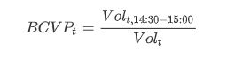
- BCVPt is the closing auction volume percentage on day t;
- Volt is the total trading volume of day t;
- Volt,14:30-15:00 is the sum of the trading volume between 14:30-15:00, representing the closing auction period in this example.
The script for implementing the formula with Python Parser is provided below:
import pandas as pd
import dolphindb as ddb

# define the function to calculate the closing auction percentage
def beforeClosingVolumePercent(trade):
    tradeTime = trade["TradeTime"].astype(ddb.TIME)
    beforeClosingVolume = trade["TradeQty"][(tradeTime >= 14:30:00.000)&(tradeTime <= 15:00:00.000)].sum()
    totalVolume = trade["TradeQty"].sum()
    res = beforeClosingVolume / totalVolume
    return pd.Series([res], ["BCVP"])

# calculate the factor on a specific day
tradeTB = loadTable("dfs://TL_Level2", "trade")
df = pd.DataFrame(tradeTB, index="Market", lazy=True)
res = df[df["TradeTime"].astype(ddb.DATE)==2023.02.01][["TradeTime", "SecurityID", "TradeQty"]].groupby(["SecurityID"]).apply(beforeClosingVolumePercent)Note:
- The function definition of
beforeClosingVolumePercentis written in Python syntax. - Since the "TradeTime" column is stored as DolphinDB TIMESTAMP type in the trade data,
tradeTime = trade["TradeTime"].astype(ddb.TIME)casts the column to the DolphinDB TIME type usingastype(). Theddbprefix must be specified before the data type name. - DolphinDB uses the
yyyy.MM.ddTHH:mm:ss.SSSformat for date/time values. For example, 14:30:00.000, 2023.02.01, 2023.02.01T14:30:00.000. tradeTB = loadTable("dfs://TL_Level2", "trade")loads the metadata (instead of the actual data) of the “trade“ table from the "dfs://TL_Level2" distributed database into the “tradeTB“ variable in memory usingloadTable().df = pd.DataFrame(tradeTB, index="Market", lazy=True)converts the DolphinDB table “tradeTB“ into a pandas DataFrame by callingpd.DataFrame(). Since tradeTB is a distributed partitioned table:- The index parameter is required - it can be specified as any column from the table as it only serves as the DataFrame’s index and will not participate in calculation;
- The lazy parameter must be set to true, which indicates the DataFrame is initialized in lazy mode, deferring computations on it for optimal performance.
Note: For more information on pd.DataFrame() and parameters, refer to the DolphinDB Python Parser manual.
- Use the
df[condition]format to retrieve data from the DataFrame by condition. For example,df[(df["TradeTime"].astype(ddb.DATE)==2023.02.01)&(df["SecurityID"]=="000001")]retrieves the “000001“ security’s data on 2023.02.01. - Retrieve only the required columns before applying
groupbyfor group calculation to minimize memory usage and reduce cost. - Perform group calculation through the
.groupby([group_by_column]).apply([function])format, which is optimized for parallel computing in the Python Parser.
1.4. Writing Results to Database
In the last section, we store the calculation results to a local variable “res“, which will be released once the session terminates. Next, we need to persist the calculation results to the partitioned table in database.
The script is as follows:
# transform res (pandas Series) to a DataFrame with 4 columns: tradetime, securityid, factorname, value
result = res.reset_index().rename(columns={"SecurityID":"securityid"})
result["tradetime"] = 2023.02.01
result = result.melt(id_vars=["tradetime", "securityid"],value_vars=["BCVP"],var_name="factorname",value_name="value")

# append results to the database table
loadTable(dbName, tbName).append!(result.to_table())

# check the number of records inserted
select count(*) from loadTable(dbName, tbName)- As the factors will be stored in the narrow format in DolphinDB, we need to convert the pandas Series “res“ to a DataFrame with four columns, tradetime, securityid, factorname and value, to match the expected schema.
- Since the previous calculation is only done for a single day (2023-02-01), the result doesn’t contain the date column. This column needs to be added manually.
- The
meltfunction reshapes the DataFrame from wide to narrow format, unpivoting the “BCVP” column into rows. When calculating multiple factors, the value_vars parameter can be modified to handle additional columns accordingly, e.g.,["factorname1", "factorname2", …]. result.to_table()converts the non-lazy DataFrame to a DolphinDB in-memory table.- The
append!function inserts the factor calculation result to the database.
2. Best Practices: Factor Storage Solutions with Python Parser
The daily volumes of factor data vary widely depending on the frequency with which the factors are calculated. In DolphinDB, data volume is a major factor deciding how data should be partitioned for optimal performance. The table below shows the volumes of factor data at various frequencies when stored in the wide format:
| Instrument Type | No. of Securities | No. of Factors | Frequency | Time Range | Volume (TB) | No. of Rows | New Volume per Day (GB) |
|---|---|---|---|---|---|---|---|
| stocks | 5,000 | 10,000 | 1 day | 11 years | 2.4 | 133.7 billion | 0.9 |
| stocks | 5,000 | 10,000 | 10 minutes | 11 years | 58.3 | 3,207.6 billion | 22.4 |
| stocks | 5,000 | 10,000 | 1 minute | 11 years | 583.4 | 32,076.0 billion | 223.5 |
| stocks | 5,000 | 1,000 | 3 seconds | 1 year | 126.8 | 5,808.0 billion | 536.4 |
| stocks | 5,000 | 1,000 | 1 second | 1 year | 380.3 | 17,424.0 billion | 1,609.3 |
| futures | 200 | 1,000 | 500 milliseconds | 1 year | 35.2 | 1,611.7 billion | 148.9 |
We have conducted performance tests to determine the optimal storage solutions for factors calculated at different frequencies. Example scripts are provided below. If you're unfamiliar with DolphinDB's database partitioning rules and how it works underneath, you can use these scripts as a quick starting point.
| Frequency | Partitioning | Partitioning Columns | sortColumns | Sort Key Entry Dimensions |
|---|---|---|---|---|
| 1 day | by year + factor name | tradetime + factorname | securityid + tradetime | 500 |
| 1 minute | by date + factor name | tradetime + factorname | securityid + tradetime | 500 |
| 10 minutes | by month + factor name | tradetime + factorname | securityid + tradetime | 500 |
| 3 seconds | by date + factor name | tradetime + factorname | securityid + tradetime | 500 |
| ticks | by date + factor name + security ID (HASH 10) | tradetime + factorname + securityid | securityid + tradetime | dimensionality reduction not required |
| 1 second | by hour+ factor name | tradetime + factorname | securityid + tradetime | 500 |
| (futures) 500 milliseconds | by date + factor name | tradetime + factorname | securityid + tradetime | 500 |
2.1. Daily Factor Storage
Sample code for creating the database and table to store factors calculated on a daily basis:
import pandas as pd
import dolphindb as ddb

dbName, tbName = "dfs://dayFactorDB", "dayFactorTB"

# Drop the database if it already exists
if existsDatabase(dbName):
    dropDatabase(dbName)

# Create a database with RANGE-based partitions (by each year) and VALUE-based partitions (by factor name)
db1 = database("", ddb.RANGE, date(datetimeAdd(1980.01M,seq(0,80)*12,'M')))
db2 = database("", ddb.VALUE, ["f1","f2"].toddb())
db = database(dbName, ddb.COMPO, [db1, db2].toddb(), engine='TSDB', atomic='CHUNK')

# create a partitioned table
schemaTB = table(array(ddb.DATE, 0) as tradetime,
                array(ddb.SYMBOL, 0) as securityid,
                array(ddb.SYMBOL, 0) as factorname,
                array(ddb.DOUBLE, 0) as value)

db.createPartitionedTable(schemaTB, tbName, partitionColumns=["tradetime", "factorname"].toddb(), compressMethods={"tradetime":"delta"}.toddb(),
                        sortColumns=["securityid", "tradetime"].toddb(), keepDuplicates=ddb.ALL, sortKeyMappingFunction=[lambda x:hashBucket(x, 500)].toddb())
2.2. 1-Minute Factor Storage
Sample code for creating the database and table to store factors calculated on a 1-minute basis:
import pandas as pd
import dolphindb as ddb

dbName, tbName = "dfs://minuteFactorDB", "minuteFactorTB"

# Drop the database if it already exists
if existsDatabase(dbName):
    dropDatabase(dbName)

# Create a database with composite VALUE-based partitions (by each day and factor name)
db1 = database("", ddb.VALUE, seq(2021.01.01, 2021.12.31))
db2 = database("", ddb.VALUE, ["f1","f2"].toddb())
db = database(dbName, ddb.COMPO, [db1, db2].toddb(), engine='TSDB', atomic='CHUNK')

# create a partitioned table
schemaTB = table(array(ddb.DATE, 0) as tradetime,
                array(ddb.SYMBOL, 0) as securityid,
                array(ddb.SYMBOL, 0) as factorname,
                array(ddb.DOUBLE, 0) as value)

db.createPartitionedTable(schemaTB, tbName, partitionColumns=["tradetime", "factorname"].toddb(), compressMethods={"tradetime":"delta"}.toddb(),
                        sortColumns=["securityid", "tradetime"].toddb(), keepDuplicates=ddb.ALL, sortKeyMappingFunction=[lambda x:hashBucket(x, 500)].toddb())
2.3. 10-Minute Factor Storage
Sample code for creating the database and table to store factors calculated on a 10-minute basis:
import pandas as pd
import dolphindb as ddb

dbName, tbName = "dfs://tenMinutesFactorDB", "tenMinutesFactorTB"

# Drop the database if it already exists
if existsDatabase(dbName):
    dropDatabase(dbName)

# Create a database with composite VALUE-based partitions (by each month and factor name)
db1 = database("", ddb.VALUE, seq(2023.01M, 2023.06M))
db2 = database("", ddb.VALUE, ["f1","f2"].toddb())
db = database(dbName, ddb.COMPO, [db1, db2].toddb(), engine='TSDB', atomic='CHUNK')

# create a partitioned table
schemaTB = table(array(ddb.DATE, 0) as tradetime,
                array(ddb.SYMBOL, 0) as securityid,
                array(ddb.SYMBOL, 0) as factorname,
                array(ddb.DOUBLE, 0) as value)

db.createPartitionedTable(schemaTB, tbName, partitionColumns=["tradetime", "factorname"].toddb(), compressMethods={"tradetime":"delta"}.toddb(),
                        sortColumns=["securityid", "tradetime"].toddb(), keepDuplicates=ddb.ALL, sortKeyMappingFunction=[lambda x:hashBucket(x, 500)].toddb())
2.4. 3-Second Factor Storage
Sample code for creating the database and table to store factors calculated on a 3-second basis:
import pandas as pd
import dolphindb as ddb

dbName, tbName = "dfs://level2FactorDB", "level2FactorTB"

# Drop the database if it already exists
if existsDatabase(dbName):
    dropDatabase(dbName)

# Create a database with composite VALUE-based partitions (by each day and factor name)
db1 = database("", ddb.VALUE, seq(2022.01.01, 2022.12.31))
db2 = database("", ddb.VALUE, ["f1","f2"].toddb())
db = database(dbName, ddb.COMPO, [db1, db2].toddb(), engine='TSDB', atomic='CHUNK')

# create a partitioned table
schemaTB = table(array(ddb.DATE, 0) as tradetime,
                array(ddb.SYMBOL, 0) as securityid,
                array(ddb.SYMBOL, 0) as factorname,
                array(ddb.DOUBLE, 0) as value)

db.createPartitionedTable(schemaTB, tbName, partitionColumns=["tradetime", "factorname"].toddb(), compressMethods={"tradetime":"delta"}.toddb(),
                        sortColumns=["securityid", "tradetime"].toddb(), keepDuplicates=ddb.ALL, sortKeyMappingFunction=[lambda x:hashBucket(x, 500)].toddb())
2.5. Tick-by-Tick Factor Storage
Sample code for creating the database and table to store factors calculated by tick:
import pandas as pd
import dolphindb as ddb

dbName, tbName = "dfs://tickFactorDB", "tickFactorTB"

# Drop the database if it already exists
if existsDatabase(dbName):
    dropDatabase(dbName)

# Create a database with VALUE-based partitions (by each day and factor name) and 10 HASH-based partitions (by security ID)
db1 = database("", ddb.VALUE, seq(2022.01.01, 2022.12.31))
db2 = database("", ddb.VALUE, ["f1","f2"].toddb())
db3 = database("", ddb.HASH, [ddb.SYMBOL, 10].toddb())
db = database(dbName, ddb.COMPO, [db1, db2, db3].toddb(), engine='TSDB', atomic='CHUNK')

# create a partitioned table
schemaTB = table(array(ddb.DATE, 0) as tradetime,
                array(ddb.SYMBOL, 0) as securityid,
                array(ddb.SYMBOL, 0) as factorname,
                array(ddb.DOUBLE, 0) as value)

db.createPartitionedTable(schemaTB, tbName, partitionColumns=["tradetime", "factorname", "securityid"].toddb(), compressMethods={"tradetime":"delta"}.toddb(),
                        sortColumns=["securityid", "tradetime"].toddb(), keepDuplicates=ddb.ALL)
2.6. 1-Second Factor Storage
Sample code for creating the database and table to store factors calculated at every second:
import pandas as pd
import dolphindb as ddb

dbName, tbName = "dfs://secondFactorDB", "secondFactorTB"

# Drop the database if it already exists
if existsDatabase(dbName):
    dropDatabase(dbName)

# Create a database with composite VALUE-based partitions (by each hour and factor name)
db1 = database("", ddb.VALUE, seq(datehour(2022.01.01T00:00:00), datehour(2022.01.31T00:00:00)))
db2 = database("", ddb.VALUE, ["f1","f2"].toddb())
db = database(dbName, ddb.COMPO, [db1, db2].toddb(), engine='TSDB', atomic='CHUNK')

# create a partitioned table
schemaTB = table(array(ddb.DATE, 0) as tradetime,
                array(ddb.SYMBOL, 0) as securityid,
                array(ddb.SYMBOL, 0) as factorname,
                array(ddb.DOUBLE, 0) as value)

db.createPartitionedTable(schemaTB, tbName, partitionColumns=["tradetime", "factorname"].toddb(), compressMethods={"tradetime":"delta"}.toddb(),
                        sortColumns=["securityid", "tradetime"].toddb(), keepDuplicates=ddb.ALL, sortKeyMappingFunction=[lambda x:hashBucket(x, 500)].toddb())
2.7. (Futures) 500-Millisecond Factor Storage
Sample code for creating the database and table to store factors calculated at every 500 milliseconds:
import pandas as pd
import dolphindb as ddb

dbName, tbName = "dfs://futuresFactorDB", "futuresFactorTB"
# Drop the database if it already exists
if existsDatabase(dbName):
    dropDatabase(dbName)

# Create a database with composite VALUE-based partitions (by each day and factor name)
db1 = database("", ddb.VALUE, seq(2021.01.01, 2021.12.31))
db2 = database("", ddb.VALUE, ["f1","f2"].toddb())
db = database(dbName, ddb.COMPO, [db1, db2].toddb(), engine='TSDB', atomic='CHUNK')

# create a partitioned table
schemaTB = table(array(ddb.DATE, 0) as tradetime,
                array(ddb.SYMBOL, 0) as securityid,
                array(ddb.SYMBOL, 0) as factorname,
                array(ddb.DOUBLE, 0) as value)

db.createPartitionedTable(schemaTB, tbName, partitionColumns=["tradetime", "factorname"].toddb(), compressMethods={"tradetime":"delta"}.toddb(),
                        sortColumns=["securityid", "tradetime"].toddb(), keepDuplicates=ddb.ALL, sortKeyMappingFunction=[lambda x:hashBucket(x, 500)].toddb())
3. Python Parser Scripts for Factors
This section contains Python Parser scripts for some common factors calculated based on market data. These scripts are provided as examples to assist you in coding with the Python Parser.
3.1. Dual Moving Average Crossover
Calculate a short term moving average (STMA) and a long term moving average (LTMA) of security price. The crossover points of the two moving averages are decision points for buying or selling securities:
- When the STMA crosses above the LTMA, it is an upward trending indicator that represents a buy signal. In code, we identify the point where the previous STMA value was below the previous LTMA value but the current STMA has moved above the current LTMA, marking it as a signal value of 1.
- When the STMA crosses below the LTMA, it indicates a downward trend and generates a sell signal. In code, we identify the point where the previous STMA value was above the previous LTMA value but the current STMA has moved below the current LTMA, marking it as a signal value of -1.
In this example, the formula for calculating the simple moving averages is used, where n represents the window size:
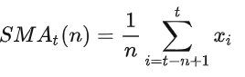
The example script uses daily market data from July 1, 2020 to July 19, 2023. You can replace the sample data with your own market data at different frequencies, such as minute and hourly levels.
Example script:
import pandas as pd
import dolphindb as ddb

# load data
df = loadTable("dfs://Daily_adj_price", "data")
df = pd.DataFrame(df, "TRADE_DATE", True)

# the function for calculating dual moving average crossovers
def signal_ma(data_chunk, short, long):
    #calculate the 5-day and 20-day moving averages, and shift the moving averages back one row to access the prior values.
    data_chunk['ma_5'] = data_chunk['CLOSE_PRICE_1'].fillna(0).rolling(int(short)).mean()
    data_chunk['ma_20'] = data_chunk['CLOSE_PRICE_1'].fillna(0).rolling(int(long)).mean()
    data_chunk['pre_ma5'] = data_chunk['ma_5'].shift(1)
    data_chunk['pre_ma20'] =  data_chunk['ma_20'].shift(1)
    # compare the averages by row using the df[condition] format to identify crossover points
    data_chunk['signal'] = 0
    data_chunk.loc[((data_chunk.loc[:,'pre_ma5']< data_chunk.loc[:,'pre_ma20'])& (data_chunk.loc[:,'ma_5'] > data_chunk.loc[:,'ma_20'])), "signal"] = 1
    data_chunk.loc[((data_chunk.loc[:,'pre_ma5']> data_chunk.loc[:,'pre_ma20']) & (data_chunk.loc[:,'ma_5'] < data_chunk.loc[:,'ma_20'])), "signal"] = -1
    return data_chunk

# generate the signals
combined_results = df.groupby('SECURITY_ID').apply(signal_ma,5,20)Note:
- The
signal_mafunction calculates the LTMA and STMA usingrolling().mean()on the adjusted closing prices, and compares the positions of the averages to identify signals at crossover points - buy (1), sell (-1), and non (0). Callingsignal_mainpd.groupby().applyallows grouped calculation of the signals for each security's price data. - The function definition for
signal_mais consistent across both Python Pandas and the Python Parser, so rewriting is not required when switching between these two environments. The Python Parser also enables more efficient batch computing through its built-in parallel execution, compared to standard Python which requires extra configuration for parallelism.
3.2. Net Buy Increase in the Best 10 Bids
Calculate the net increase in bid value within the best 10 bids, i.e., the sum of all value changes in these bids. In this example, the calculation is based on the level 2 snapshot data.
The formula is as follows:
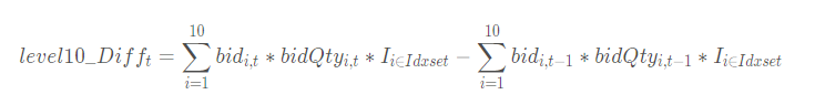
- level10_Difft is the net buy increase of the best 10 bids at time t;
- bidi,t is the ith best bid price at time t;
- bidQtyi,t is the bid quantity of the ith best bid price at time t;
- the indicator function I indicates whether the bid price is within the best 10 range at the time t. The expression of I is as follows:
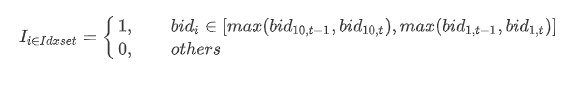
Finally, sum up the net buy increases over the time period of n (the window size).
Example script:
import pandas as pd
import dolphindb as ddb

# function definition for the factor
def level10Diff(df, lag=20):
    temp = df[["TradeTime", "SecurityID"]]
    temp["bid"] = df["BidPrice"].fillna(0)
    temp["bidAmt"] = df["BidOrderQty"].fillna(0) * df["BidPrice"].fillna(0)
    temp["prevbid"] = temp["bid"].shift(1).fillna(0)
    temp["prevbidAmt"] = temp["bidAmt"].shift(1).fillna(0)
    temp["bidMin"] = temp["bid"].apply("min")
    temp["bidMax"] = temp["bid"].apply("max")
    temp["prevbidMin"] = temp["bidMin"].shift(1).fillna(0)
    temp["prevbidMax"] = temp["bidMax"].shift(1).fillna(0)
    temp["pmin"] = temp[["bidMin", "prevbidMin"]].max(axis=1)
    temp["pmax"] = temp[["bidMax", "prevbidMax"]].max(axis=1)
    amount = temp["bidAmt"]*((temp["bid"]>=temp["pmin"])&(temp["bid"]<=temp["pmax"]))
    lastAmount = temp["prevbidAmt"]*((temp["prevbid"]>=temp["pmin"])&(temp["prevbid"]<=temp["pmax"]))
    temp["amtDiff"] = amount.apply("sum") - lastAmount.apply("sum")
    temp["amtDiff"] = temp["amtDiff"].rolling(lag, 1).sum()
    return temp[["TradeTime", "SecurityID", "amtDiff"]].fillna(0)

# calculate the factor for a specific security on a specific day
snapshotTB = loadTable("dfs://TL_Level2", "snapshot")
df = pd.DataFrame(snapshotTB, index="Market", lazy=True)
df = df[(df["TradeTime"].astype(ddb.DATE)==2023.02.01)&(df["SecurityID"]=="000001")]
res = level10Diff(df.compute(), 20)

# calculate the factor on the data of a specific day
snapshotTB = loadTable("dfs://TL_Level2", "snapshot")
df = pd.DataFrame(snapshotTB, index="Market", lazy=True)
res = df[df["TradeTime"].astype(ddb.DATE)==2023.02.01][["TradeTime", "SecurityID", "BidPrice", "BidOrderQty"]].groupby(["SecurityID"]).apply(lambda x:level10Diff(x, 20))Note:
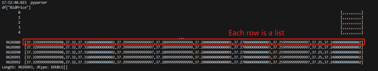
- The level 2 snapshot data includes many columns holding similar types of data, such as the best 10 bid prices and quantities. Instead of having 10 separate columns for each bid price or quantity, they are stored more efficiently in DolphinDB as array vectors - 2D vectors where each element is a variable-length vector. In this example, "BidPrice" and "BidOrderQty" are two array vector columns holding the top 10 bid prices and quantities, respectively.
- When a DolphinDB array vector column is converted into a pandas DataFrame column, each of its element becomes a List.
- The Python Parser supports basic arithmetic operations and comparisons on DataFrame columns converted from DolphinDB array vectors. For example,
df["BidOrderQty"].fillna(0) * df["BidPrice"].fillna(0)multiplies two columns. For more complex logic, use theapplyfunction. For example,temp["bid"].apply("min")gets the minimum per row of the “bid“ column. - Built-in functions like
max/min/sumcan be called in two forms when used inapply:- Passing the name as a string, e.g.
temp["bid"].apply("max"), will callSeries.max()first if it exists, falling back to the DolphinDB built-in functionmax(). This call form is recommended in most cases. - Passing the actual function, e.g.
temp["bid"].apply(max), will directly execute the DolphinDB built-in functionmax().
- Passing the name as a string, e.g.
.shift(1)returns the previous value for each row..rolling().sum()sums the value changes in best 10 bids over the specified timeframe.- The following steps are similar to those described in the "Calculating the Closing Auction Percentage" example. For details, refer to the previous notes:
loadTable()loads the metadata of the “snapshot” table from the database into memory;pd.DataFrame()converts the table to a pandas DataFrame;df[condition]filters DataFrame data via conditions;- To minimize memory usage, only the required columns are selected before grouped calculation, which is achieved through
.groupby([group_by_column]).apply([function]).
- The "snapshotTB" DataFrame is initialized in lazy mode, disabling direct modifications on itself. In
res = level10Diff(df.compute(), 20),df.compute()converts the DataFrame into non-lazy mode, enabling immediate execution of operations liketemp["bid"]=df["BidPrice"].fillna(0)to execute immediately. Otherwise, the error "Lazy DataFrame does not support updating values" will be raised. For more information on lazy DataFrames, refer to the DolphinDB Python Parser manual.
3.3. Price Sensitivity to Order Flow Imbalance
Calculate the regression coefficient between security price changes and the quantity imbalance at the best bid vs ask prices. In this example, the calculation is based on the level 2 snapshot data.
The regression model is as follows:
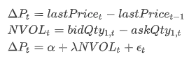
- ΔPt is the price change from previous price to current price at time t
- NVOLt is the difference between bid quantity and ask quantity at the best price at time t
- α is the intercept, λ is the regression coefficient (i.e., the factor we calculate), and εt is the residual at time t.
Example script:
import pandas as pd
import dolphindb as ddb

# function definition for the factor
def priceSensitivityOrderFlowImbalance(df):
    deltaP = 10000*df["LastPrice"].diff().fillna(0)
    bidQty1 = df["BidOrderQty"].values[0]
    askQty1 = df["OfferOrderQty"].values[0]
    NVOL = bidQty1 - askQty1
    res = beta(deltaP.values, NVOL)
    return pd.Series([res], ["priceSensitivityOrderFlowImbalance"])

# calculate the factor for a specific security on a specific day
snapshotTB = loadTable("dfs://TL_Level2", "snapshot")
df = pd.DataFrame(snapshotTB, index="Market", lazy=True)
df = df[(df["TradeTime"].astype(ddb.DATE)==2023.02.01)&(df["SecurityID"]=="000001")]
res = priceSensitivityOrderFlowImbalance(df.compute())

# calculate the factor on a specific day
snapshotTB = loadTable("dfs://TL_Level2", "snapshot")
df = pd.DataFrame(snapshotTB, index="Market", lazy=True)
res = df[df["TradeTime"].astype(ddb.DATE)==2023.02.01][["SecurityID", "LastPrice", "BidOrderQty", "OfferOrderQty"]].groupby(["SecurityID"]).apply(priceSensitivityOrderFlowImbalance) Note:
- In this example, "BidOrderQty" and "OfferOrderQty" are two array vector columns holding the quantities at the best 10 bid/ask prices, respectively. When these array vector columns are converted into pandas DataFrame columns, each array vector element becomes a List.
- In the earlier example, we use
apply()to execute pandas functions or lambda expressions on DataFrame columns. Alternatively, we can useSeries.values()to transform a Series into a DolphinDB vector, enabling the application of DolphinDB's built-in functions. DolphinDB provides flexible slicing techniques and built-in functions with great performance for array vectors. In this example,df["BidOrderQty"].values[0]converts the "BidOrderQty" column into DolphinDB array vector and retrieves its first column. diff(1)calculates the first-order difference.- The “LastPrice” column is stored using the DOUBLE data type. With
deltaP = 10000*df["LastPrice"].diff().fillna(0), the price change is magnified by 10,000 times for clarity, as the order of magnitude between the price and quantity differs greatly. - The Python Parser currently does not support data analysis packages like statsmodels and sklearn. This means there is no built-in function for direct regression calculation. As a workaround, however, we can convert a Pandas Series into a DolphinDB vector using
Series.values(). The DolphinDB vector can then leverage native functions likebeta()to run regressions. In this example,beta(deltaP.values, NVOL). - The following steps are similar to those described in the "Calculating the Closing Auction Percentage" example. For details, refer to the previous notes:
loadTable()loads the metadata of the “snapshot” table from the database into memory;pd.DataFrame()converts the table to a pandas DataFrame;df[condition]filters DataFrame data via conditions;- To minimize memory usage, only the required columns are selected before grouped calculation, which is achieved through
.groupby([group_by_column]).apply([function]).
3.4. Active Buy Trade Volume Ratio
Calculate the proportion of trade volume from active buy orders out of the total trade volume. In this example, the calculation is based on the tick trade data.
The formulae are as follows:
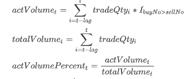
- tradeQtyi is the trade quantity of the ith order;
- actVolumet is the sum of all trade quantities of active buy orders out of the last lag active buy orders until the tth order;
- totalVolumet is the sum of all trade quantities of the last lag orders until the tth order;
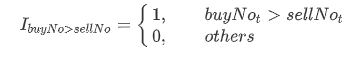
- I is the indicator function which is defined as follows:
Example script:
import pandas as pd
import dolphindb as ddb

# function definition for the factor
def actVolumePercent(trade, lag):
    res = trade[["TradeTime", "SecurityID"]]
    actVolume = (trade["TradeQty"]*(trade['BidApplSeqNum'] > trade['OfferApplSeqNum'])).rolling(lag).sum()
    totalVolume = trade["TradeQty"].rolling(lag).sum()
    res["actVolumePercent"] = actVolume/totalVolume
    return res

# calculate the factor for a specific security on a specific day
tradeTB = loadTable("dfs://TL_Level2", "trade")
df = pd.DataFrame(tradeTB, index="Market", lazy=True)
df = df[(df["TradeTime"].astype(ddb.DATE)==2023.02.01)&(df["SecurityID"]=="000001")]
res = actVolumePercent(df.compute(), 60)

# calculate the factor on a specific day
tradeTB = loadTable("dfs://TL_Level2", "trade")
df = pd.DataFrame(tradeTB, index="Market", lazy=True)
res = df[df["TradeTime"].astype(ddb.DATE)==2023.02.01][["TradeTime", "SecurityID", "TradeQty", "BidApplSeqNum", "OfferApplSeqNum"]].groupby(["SecurityID"]).apply(lambda x: actVolumePercent(x, 60))Note:
trade['BidApplSeqNum'] > trade['OfferApplSeqNum']identifies the active buy orders.rolling(lag).sum()returns the sum of all trade quantities of the last lag orders;- The following steps are similar to those described in the "Calculating the Closing Auction Percentage" example. For details, refer to the previous notes:
loadTable()loads the metadata of the “trade” table from the database into memory;pd.DataFrame()converts the table to a pandas DataFrame;df[condition]filters DataFrame data via conditions;- To minimize memory usage, only the required columns are selected before grouped calculation, which is achieved through
.groupby([group_by_column]).apply([function]).
- The "df" DataFrame is initialized in lazy mode, disabling direct modification on itself. However, the definition of
actVolumePercent()includes the operationres["actVolumePercent"] = actVolume/totalVolume. This means directly executingactVolumePercent(df, 60)will raise the error "Lazy DataFrame does not support updating values." To resolve this,df.compute()is called to convert the DataFrame into non-lazy mode, enabling immediate operations.
3.5. Morning Session Bid-Ask Order Quantity Ratio
Calculate the logarithm of the ratio between the average order quantity for bid orders and ask orders during the morning trading session. In this example, the calculation is based on the level 2 tick-by-tick order data.
The formulae are as follows:
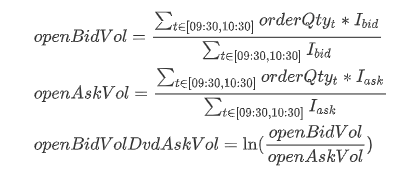
- openBidVol is the average order quantity for bid orders during the morning session;
- openAskVol is the average order quantity for ask orders during the morning session;
- orderQtyt is the order quantity at time t;
- Ibid is an indicator function which returns 1 for bid orders and 0 for ask orders. In contrast, Iask returns 1 for ask orders and 0 for bid orders.
Example script:
import pandas as pd
import dolphindb as ddb

# function definition for the factor
def openBidVolDvdAskVol(df):
    tradeTime = df["TradeTime"].astype(ddb.TIME)
    openBidVolume = df["OrderQty"][(tradeTime >= 09:30:00.000)&(tradeTime <= 10:30:00.000)&((df["Side"]=="1")|(df["Side"]=="B"))].mean()
    openAskVolume = df["OrderQty"][(tradeTime >= 09:30:00.000)&(tradeTime <= 10:30:00.000)&((df["Side"]=="2")|(df["Side"]=="S"))].mean()
    if((openBidVolume>0)&(openAskVolume>0)):
        res = log(openBidVolume / openAskVolume)
    else:
        res = None
    return pd.Series([res], ["openBidVolDvdAskVol"])

# calculate the factor for a specific security on a specific day
orderTB = loadTable("dfs://TL_Level2", "entrust")
df = pd.DataFrame(orderTB, index="Market", lazy=True)
df = df[(df["TradeTime"].astype(ddb.DATE)==2023.02.01)&(df["SecurityID"]=="000001")]
res = openBidVolDvdAskVol(df)

# calculate the factor on a specific day
orderTB = loadTable("dfs://TL_Level2", "entrust")
df = pd.DataFrame(orderTB, index="Market", lazy=True)
df = df[df["TradeTime"].astype(ddb.DATE)==2023.02.01]
res = df[df["TradeTime"].astype(ddb.DATE)==2023.02.01][["TradeTime", "SecurityID", "OrderQty", "Side"]].groupby(["SecurityID"]).apply(openBidVolDvdAskVol)Note:
- Since the "TradeTime" column is stored as DolphinDB TIMESTAMP type in the trade data,
tradeTime = trade["TradeTime"].astype(ddb.TIME)casts the column to the DolphinDB TIME type usingastype(). Theddbprefix must be specified before the data type name. - DolphinDB uses the
yyyy.MM.ddTHH:mm:ss.SSSformat for date/time values. For example, 14:30:00.000, 2023.02.01, 2023.02.01T14:30:00.000. - Data from different exchanges can use varying markers to denote the direction of orders. In this example, one exchange marks bids as "B" and asks as "S", while another exchange uses "1" for bids and "2" for asks. To handle this, the code lines with the
mean()calculation contains an OR (|) logic check to capture both exchanges' bid/ask orders. if((openBidVolume>0)&(openAskVolume>0))performs a validation check to handle cases where no orders are placed during the morning trading session.- The following steps are similar to those described in the "Calculating the Closing Auction Percentage" example. For details, refer to the previous notes:
loadTable()loads the metadata of the “entrust” table from the database into memory;pd.DataFrame()converts the table to a pandas DataFrame;df[condition]filters DataFrame data via conditions;- To minimize memory usage, only the required columns are selected before grouped calculation, which is achieved through
.groupby([group_by_column]).apply([function]).
3.6. Volume-Weighted Average Order Price
Calculate a volume-weighted average price (VWAP) over multiple orders. In this example, the level 2 tick-by-tick order data is used.
The formula is as follows:
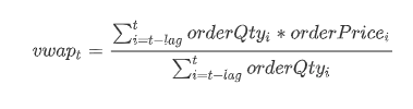
- vwapt is the volume-weighted average price over the next lag orders starting from time t;
- orderQtyi is the order quantity at time i;
- orderPricei is the order price at time i.
Example script:
import pandas as pd
import dolphindb as ddb

# function definition for the factor
def volumeWeightedAvgPrice(df, lag):
    res = df[["TradeTime", "SecurityID"]]
    totalAmount = (df["OrderQty"]*df["Price"]).rolling(lag).sum()
    totalVolume = df["OrderQty"].rolling(lag).sum()
    res["volumeWeightedAvgPrice"] = totalAmount / totalVolume
    return res

# calculate the factor for a specific security on a specific day
orderTB = loadTable("dfs://TL_Level2", "entrust")
df = pd.DataFrame(orderTB, index="Market", lazy=True)
df = df[(df["TradeTime"].astype(ddb.DATE)==2023.02.01)&(df["SecurityID"]=="000001")]
res = volumeWeightedAvgPrice(df.compute(), 60)

# calculate the factor on a specific day
orderTB = loadTable("dfs://TL_Level2", "entrust")
df = pd.DataFrame(orderTB, index="Market", lazy=True)
res = df[df["TradeTime"].astype(ddb.DATE)==2023.02.01][["TradeTime", "SecurityID", "OrderQty", "Price"]].groupby(["SecurityID"]).apply(lambda x: volumeWeightedAvgPrice(x, 60))Note:
rolling(lag).sum()is called twice to calculate the total order prices and total order quantity over the last lag orders, respectively.- The following steps are similar to those described in the "Calculating the Closing Auction Percentage" example. For details, refer to the previous notes:
loadTable()loads the metadata of the “entrust” table from the database into memory;pd.DataFrame()converts the table to a pandas DataFrame;df[condition]filters DataFrame data via conditions;- To minimize memory usage, only the required columns are selected before grouped calculation, which is achieved through
.groupby([group_by_column]).apply([function]).
- The "df" DataFrame is initialized in lazy mode, disabling direct modification on itself. However, the definition of
volumeWeightedAvgPriceincludes the operationres["orderWeightPrice"] = totalAmount/totalVolume. This means directly executingvolumeWeightedAvgPrice(df, 60)will raise the error "Lazy DataFrame does not support updating values." To resolve this,df.compute()is called to convert the DataFrame into non-lazy mode, enabling immediate operations.
4. Performance Testing
4.1. Environment
| CPU | Intel(R) Xeon(R) Gold 5220R CPU @ 2.20GHz |
|---|---|
| Number of Logical CPU Cores | 24 |
| Memory | 256 GB |
| OS | CentOS Linux release 7.9.2009 (Core) |
4.2. Test Results
The test data used is as follows:
- One day’s level-2 data for a single exchange in 2023:
- Snapshot data: 24,313,086 rows × 62 columns [approximately 20.6 GB]
- Tick-by-tick trade data: 108,307,125 rows × 19 columns [approximately 11.0 GB]
- Tick-by-tick order data : 141,182,534 rows × 16 columns [approximately 11.6 GB]
| Test Data | Factor | Execution Time with Python Parser | Execution Time with DolphinDB Scripts | Execution Time with Python | Execution Time Ratio: DolphinDB Scripts/ Python Parser | Execution Time Ratio: Python /Python Parser |
|---|---|---|---|---|---|---|
| Daily OHLC Data | Dual moving average crossover (single stock) | 10.88 ms | 9.07 ms | 30 ms | 0.836 | 2.757 |
| Daily OHLC Data | Dual moving average crossover (market) | 1.1 s | 0.566 s | 14.01 s | 0.515 | 12.74 |
| Snapshot | Net buy increase in the best 10 bids | 4.3 s | 1.4 s | 49.4 s | 0.326 | 11.488 |
| Snapshot | Price sensitivity to order flow imbalance | 2.8 s | 0.34 s | 25.5 s | 0.019 | 9.107 |
| Tick-by-Tick Trade Data | Active buy trade volume ratio | 6.9 s | 1.2 s | 52.9 s | 0.174 | 7.667 |
| Tick-by-Tick Trade Data | Closing auction percentage | 4.1 s | 0.31 s | 19.6 s | 0.076 | 4.780 |
| Tick-by-Tick Order Data | Morning session bid-ask order quantity ratio | 5.8 s | 0.64 s | 21.1 s | 0.110 | 3.638 |
| Tick-by-Tick Order Data | Volume-weighted average order price | 7.2 s | 1.4 s | 77.2 s | 0.194 | 10.722 |
5. Conclusion
The DolphinDB Python Parser supports core Python syntax while allowing DolphinDB-specific syntax extensions. Unlike the DolphinDB Python API, the Python Parser can directly access data stored in DolphinDB databases without network transfer costs. It also enables parallel computation when executing functions like .groupby(), boosting performance. Compared to DolphinDB's own scripting language, the Python Parser is more accessible to Python programmers through its compatibility with Python syntax.
This tutorial demonstrates using the Python Parser for common factor development tasks in quantitative analysis. It covers storage solutions for factors calculated at different frequencies, along with example scripts calculating popular factors from different market data sources. Performance tests indicate that factor computation using the Python Parser is more than 5 times faster than the standard Python multiprocessing framework across most scenarios described in this tutorial.
6. Appendices
Test data: tradeData.zip
Factor scripts (DolphinDB):
Factor scripts (Python Parser)