Market Data Replay
Tick data replay is critical for high-frequency trading strategy development. This tutorial introduces data replay in DolphinDB and gives detailed examples. An important feature is to ensure that data from multiple data sources (for examples, quotes and trades) is replayed to multiple tables in chronological order.
1. Replay Types
DolphinDB's replay tools replay data at a certain rate to simulate real-time ingestion of stream data. To replay an in-memory table, use function replay. When replaying a DFS table with a large amount of data, if you load all data into memory first, you may have an out-of-memory problem. In such cases, you can use function replayDS to generate multiple data sources based on date (or date and time) and then use function replay to replay these data sources sequentially.
There are 3 mapping types between the input table(s) and output table(s) : 1-to-1, N-to-1, and N-to-N.
1.1. 1-to-1 Replay
Replay a single table to a target table with the same schema.
The following example replays data from table "trade" to table "tradeStream" at a rate of 10,000 records per second.
tradeDS = replayDS(sqlObj=<select * from loadTable("dfs://trade", "trade") where Date = 2020.12.31>, dateColumn=`Date, timeColumn=`Time)
replay(inputTables=tradeDS, outputTables=tradeStream, dateColumn=`Date, timeColumn=`Time, replayRate=10000, absoluteRate=true)
1.2. N-to-N Replay
Replay multiple tables to target tables. Each of the output tables corresponds to an input table and has the same schema as the corresponding input table.
The following example replays data from three tables ("order", "trade", "snapshot") to three target tables ("orderStream", "tradeStream", "snapshotStream") at a rate of 10,000 records per second:
orderDS = replayDS(sqlObj=<select * from loadTable("dfs://order", "order") where Date = 2020.12.31>, dateColumn=`Date, timeColumn=`Time)
tradeDS = replayDS(sqlObj=<select * from loadTable("dfs://trade", "trade") where Date = 2020.12.31>, dateColumn=`Date, timeColumn=`Time)
snapshotDS = replayDS(sqlObj=<select * from loadTable("dfs://snapshot", "snapshot") where Date =2020.12.31>, dateColumn=`Date, timeColumn=`Time)
replay(inputTables=[orderDS, tradeDS, snapshotDS], outputTables=[orderStream, tradeStream, snapshotStream], dateColumn=`Date, timeColumn=`Time, replayRate=10000, absoluteRate=true)
1.3. N-to-1 Replay
Replay multiple tables to one table. Prior to version 1.30.7/2.00.5, replay only supports inputting tables with the same schema, which is called homogeneous replay. Starting from version 1.30.17/2.00.5, heterogeneous replay is supported to replay multiple data sources with different schemata to the same output table.
Different from N-to-1 homogeneous replay and N-to-N replay, the inputTables of heterogeneous replay is a dictionary. The key of the dictionary is the unique identifier of the input table, and the value is the table object or data source.
The following example replays data from three tables ("order", "trade", "snapshot") with different schemata to one target table ("messageStream") at a rate of 10,000 records per second:
orderDS = replayDS(sqlObj=<select * from loadTable("dfs://order", "order") where Date = 2020.12.31>, dateColumn=`Date, timeColumn=`Time)
tradeDS = replayDS(sqlObj=<select * from loadTable("dfs://trade", "trade") where Date = 2020.12.31>, dateColumn=`Date, timeColumn=`Time)
snapshotDS = replayDS(sqlObj=<select * from loadTable("dfs://snapshot", "snapshot") where Date =2020.12.31>, dateColumn=`Date, timeColumn=`Time)
inputDict = dict(["order", "trade", "snapshot"], [orderDS, tradeDS, snapshotDS])
replay(inputTables=inputDict, outputTables=messageStream, dateColumn=`Date, timeColumn=`Time, replayRate=10000, absoluteRate=true)
The output table "messageStream" has the following schema:
| name | typeString | comment |
|---|---|---|
| timestamp | TIMESTAMP | The timestamp specified by dateColumn/timeColumn |
| source | SYMBOL | The unique identifier of data sources ("order", "trade", "snapshot") |
| msg | BLOB | The serialized result of each replayed record (in binary format) |
Part of the table "messageStream":
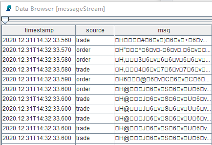
Such schema guarantees multiple data sources are replayed in strict chronological order, and replayed data (stored in the same table "messageStream") can also be processed by a single thread in chronological order.
To process data in table "messageStream" (e.g., calculating metrics), deserialize the replayed records (column "msg" above). DolphinDB supports deserializing data in heterogeneous stream tables with built-in function streamFilter or DolphinDB APIs.
2. Replay Trades & Quotes With Different Schemata
Examples of N-to-1 heterogenous replay in this chapter show how to replay and process market data (trades, quotes, snapshot) in DolphinDB.
2.1. Trades & Quotes Replay and Consumption
The figure below is the market data replay flowchart:
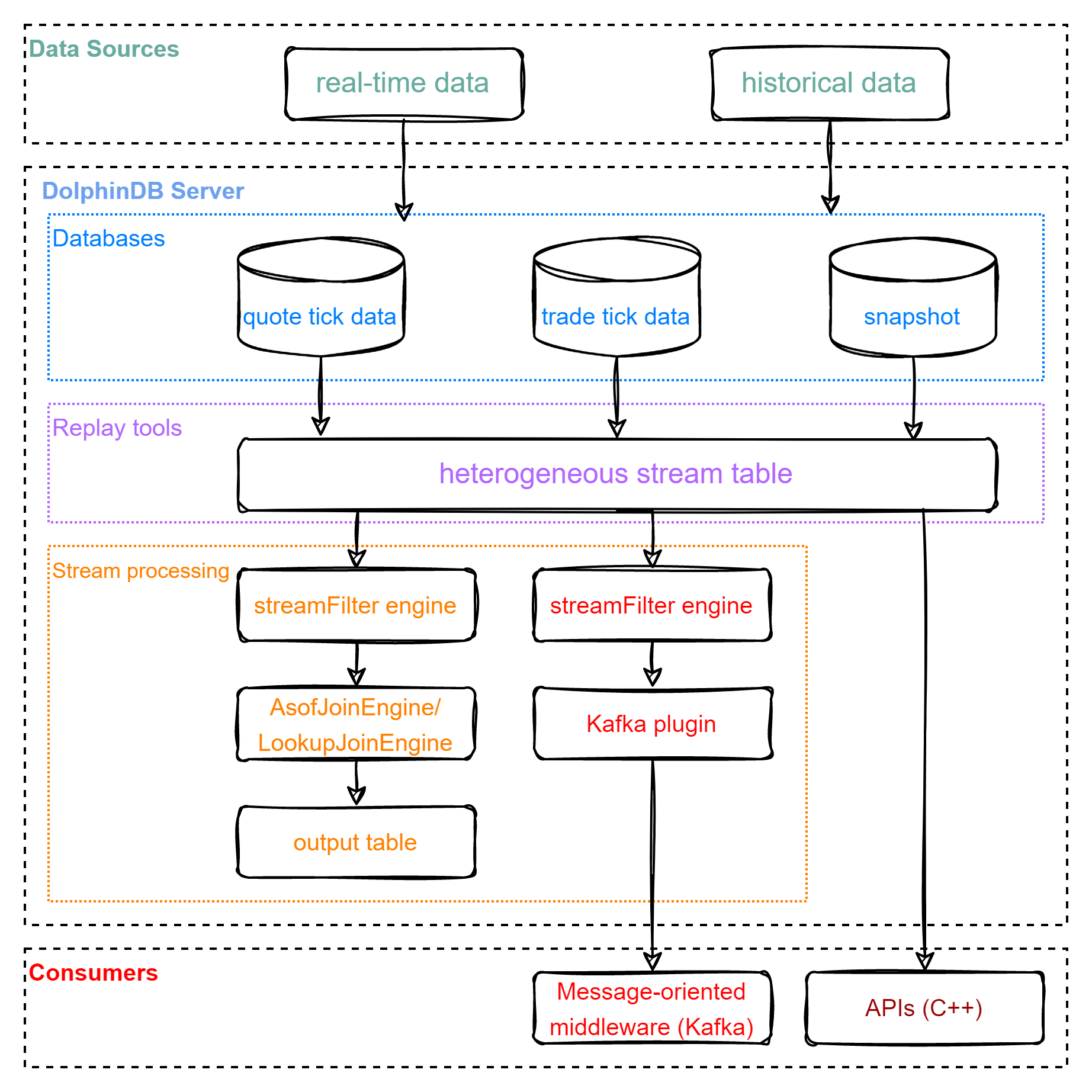
The replay processing has two major phases: replay and consumption.
(1) Replay data stored in multiple databases to a stream table in DolphinDB server; (2) The stream table can be consumed with: - DolphinDB built-in streaming engines to calculate metrics; - Kafka (message-oriented middleware) through DolphinDB Kafka plugin; - DolphinDB APIs.
2.2. Test Data
The example in this tutorial replays Shanghai Stock Exchange market data of a given day.
The following chart displays the data we use in the example (which is stored in TSDB databases):
| Data | The number of columns | The number of records | Data size | Table | Partitioning scheme | Sort column |
|---|---|---|---|---|---|---|
| quote tick data (dfs://order) | 20 | 49018552 | 6.8G | order | VALUE: trade date; HASH: [SYMBOL, 20] | Time; SecurityID |
| trade tick data(dfs://trade) | 15 | 43652718 | 3.3G | trade | VALUE: trade date; HASH: [SYMBOL, 20] | Time; SecurityID |
| snapshots of level 2 tick data(dfs://snapshot) | 55 | 8410359 | 4.1G | snapshot | VALUE: trade date; HASH: [SYMBOL, 20] | Time; SecurityID |
2.3. Trades & Quotes Replay
We use DolphinDB GUI to implement all scripts in this example. For details about test environment configuration, see "Development Environment".
In this section, we replay three tables with different schemata to a single stream table. See full scripts in 01. MarketDataReplay.
Define the shared stream table "messageStream".
colName = `timestamp`source`msg
colType = [TIMESTAMP,SYMBOL, BLOB]
messageTemp = streamTable(1000000:0, colName, colType)
enableTableShareAndPersistence(table=messageTemp, tableName="messageStream", asynWrite=true, compress=true, cacheSize=1000000, retentionMinutes=1440, flushMode=0, preCache=10000)
messageTemp = NULL
Replay three tables ("order", "trade", "snapshot") to the stream table "messageStream" and execute the replay function as a background job using function
submitJob.timeRS = cutPoints(09:15:00.000..15:00:00.000, 100) orderDS = replayDS(sqlObj=<select * from loadTable("dfs://order", "order") where Date = 2020.12.31>, dateColumn=`Date, timeColumn=`Time, timeRepartitionSchema=timeRS) tradeDS = replayDS(sqlObj=<select * from loadTable("dfs://trade", "trade") where Date = 2020.12.31>, dateColumn=`Date, timeColumn=`Time, timeRepartitionSchema=timeRS) snapshotDS = replayDS(sqlObj=<select * from loadTable("dfs://snapshot", "snapshot") where Date =2020.12.31>, dateColumn=`Date, timeColumn=`Time, timeRepartitionSchema=timeRS) inputDict = dict(["order", "trade", "snapshot"], [orderDS, tradeDS, snapshotDS]) submitJob("replay", "replay stock market", replay, inputDict, messageStream, `Date, `Time, , , 3)The above script has tuned the replay function with the following parameters:
- timeRepartitionSchema (of
replayDS) deliminates multiple data sources based on "timeColumn" within each date. The SQL query job is broken down into multiple tasks.
With parameter timeRepartitionSchema specified, each table in the above example is divided into 100 data sources based on the "Time" column within date "2020.12.31". Each data source is loaded by a query task, which prevents the out-of-memory problem.
If timeRepartitionSchema is not specified, the SQL query is as follows:
select * from loadTable("dfs://order", "order") where Date = 2020.12.31 order by TimeIf timeRepartitionSchema is specified, the SQL query is as follows:
select * from loadTable("dfs://order", "order") where Date = 2020.12.31, 09:15:00.000 <= Time < 09:18:27.001 order by Time- parallelLevel (of
replay) is the number of threads loading data into memory from data sources. The default value is 1.
With parallelLevel parameter set to 3 in the above example, multiple data sources are loaded by three threads in parallel, thus improving performance of query.
After submitting the replay job, check its status with the
getRecentJobsfunction. In case you need to cancel the replay, use thecancelJobfunction with the job ID obtained fromgetRecentJobs.If there is no available data, you can get started with the sample data listed in Appendices.
Replace "/yourDataPath/" in the following script with path where csv files are stored.
orderDS = select * from loadText("/yourDataPath/replayData/order.csv") order by Time tradeDS = select * from loadText("/yourDataPath/replayData/trade.csv") order by Time snapshotDS = select * from loadText("/yourDataPath/replayData/snapshot.csv") order by Time inputDict = dict(["order", "trade", "snapshot"], [orderDS, tradeDS, snapshotDS]) submitJob("replay", "replay text", replay, inputDict, messageStream, `Date, `Time, , , 1)- timeRepartitionSchema (of
2.4. Replayed Data Consumption
2.4.1. Consuming With DolphinDB Built-in Streaming Engine
In the following example, we define asof join engine that returns the as of join result of trade and snapshot (from "messageStream") to calculate the transaction cost. See full scripts in 02. CalculateTxnCost_asofJoin.
Define the shared stream table "prevailingQuotes" as the output table.
colName = `TradeTime`SecurityID`Price`TradeQty`BidPX1`OfferPX1`Spread`SnapshotTime
colType = [TIME, SYMBOL, DOUBLE, INT, DOUBLE, DOUBLE, DOUBLE, TIME]
prevailingQuotesTemp = streamTable(1000000:0, colName, colType)
enableTableShareAndPersistence(table=prevailingQuotesTemp, tableName="prevailingQuotes", asynWrite=true, compress=true, cacheSize=1000000, retentionMinutes=1440, flushMode=0, preCache=10000)
prevailingQuotesTemp = NULL
Define the asof join engine. The user-defined function createSchemaTable is used to get the table schema and use it as a parameter of createAsofJoinEngine.
def createSchemaTable(dbName, tableName){
	schema = loadTable(dbName, tableName).schema().colDefs
	return table(1:0, schema.name, schema.typeString)
}
tradeSchema = createSchemaTable("dfs://trade", "trade")
snapshotSchema = createSchemaTable("dfs://snapshot", "snapshot")

joinEngine=createAsofJoinEngine(name="tradeJoinSnapshot", leftTable=tradeSchema, rightTable=snapshotSchema, outputTable=prevailingQuotes, metrics=<[Price, TradeQty, BidPX1, OfferPX1, abs(Price-(BidPX1+OfferPX1)/2), snapshotSchema.Time]>, matchingColumn=`SecurityID, timeColumn=`Time, useSystemTime=false, delayedTime=1)
For each stock, the asof join engine matches each record of table "trade" with the most recent record from table "snapshot", and then you can calculate transaction costs with the price and quote.
Considering the common practice, we set parameter useSystemTime to false in the above script to perform asof join based on the "timeColumn".
Alternatively, you can set parameter useSystemTime to true or use lookup join engine (see full script in 03. CalculateTxnCost_lookUpJoin).
Define a stream filter engine.
def appendLeftStream(msg){
	tempMsg = select * from msg where Price > 0 and Time>=09:30:00.000
	getLeftStream(getStreamEngine(`tradeJoinSnapshot)).tableInsert(tempMsg)
}
filter1 = dict(STRING,ANY)
filter1["condition"] = "trade"
filter1["handler"] = appendLeftStream
filter2 = dict(STRING,ANY)
filter2["condition"] = "snapshot"
filter2["handler"] = getRightStream(getStreamEngine(`tradeJoinSnapshot))
schema = dict(["trade", "snapshot"], [tradeSchema, snapshotSchema])
engine = streamFilter(name="streamFilter", dummyTable=messageStream, filter=[filter1, filter2], msgSchema=schema)
The ingested data is deserialized according to parameter msgSchema and processed based on the handler of parameter filter. The serial execution of multiple handlers guarantees the strict chronological order of data processing.
The "messageStream" table is splitted into two streams. Table "trade" is processed with user-defined function appendLeftStream before it is ingested into asof join engine as the left table. Table "snapshot" is directly ingested into asof join engine as the right table.
Subscribe to the replayed data (heterogeneous stream table)
subscribeTable(tableName="messageStream", actionName="tradeJoinSnapshot", offset=-1, handler=engine, msgAsTable=true, reconnect=true)With parameter offset set to -1, the subscription starts with the next new message. To consume data from the first record, it is recommended to submit the subscription first and replay as background job afterwards.
Check the result
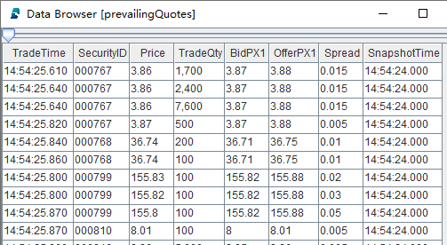
Within each group of the matchingColumn ("SecurityID"), the order of the output is the same as the order of the input.
2.4.2. Consuming with Kafka
In the following example, we send subscribed table ("messageStream") to Kafka consumer.
You need to start Kafka server and install DolphinDB Kafka Plugin first. For details about test environment configuration, see "Development Environment". For full scripts about this example, see 04. SendMsgToKafka.
Load Kafka Plugin and define a Kafka producer
loadPlugin("/DolphinDB/server/plugins/kafka/PluginKafka.txt")
go
producerCfg = dict(STRING, ANY)
producerCfg["metadata.broker.list"] = "localhost"
producer = kafka::producer(producerCfg)
Replace the loadPlugin path and you can modify producerCfg as required. Kafka and DolphinDB server are on the same server, thus, the metadata.broker.list parameter is set as localhost.
Define the function to send messages to Kafka topic
def sendMsgToKafkaFunc(dataType, producer, msg){
	startTime = now()
	try {
		kafka::produce(producer, "topic-message", 1, msg, true)
		cost = now() - startTime
		writeLog("[Kafka Plugin] Successed to send" + dataType + ":" + msg.size() + "rows," + cost + "ms.")
	}
	catch(ex) {writeLog("[Kafka Plugin] Failed to send msg to kafka with error:" +ex)}
}
Function
kafka::producesends messages of any table schema in json format to specified Kafka topic. You can check the status of a batch of messages sent previously with thewriteLogfunction.You can consume subscribed data after sending messages to Kafka.
Define a stream filter engine
filter1 = dict(STRING,ANY)
filter1["condition"] =  "order"
filter1["handler"] = sendMsgToKafkaFunc{"order", producer}
filter2 = dict(STRING,ANY)
filter2["condition"] = "trade"
filter2["handler"] = sendMsgToKafkaFunc{"trade", producer}
filter3 = dict(STRING,ANY)
filter3["condition"] = "snapshot"
filter3["handler"] = sendMsgToKafkaFunc{"snapshot", producer}

schema = dict(["order","trade", "snapshot"], [loadTable("dfs://order", "order"), loadTable("dfs://trade", "trade"), loadTable("dfs://snapshot", "snapshot")])

engine = streamFilter(name="streamFilter", dummyTable=messageStream, filter=[filter1, filter2, filter3], msgSchema=schema)
The ingested data is deserialized according to parameter msgSchema and processed based on the handler of parameter filter. The serial execution of multiple handlers guarantees the strict chronological order of data processing.
sendMsgToKafka{"order", producer} is a partial application of functional programming, which fixes part of the parameters of the sendMsgToKafka function to generate a new function with fewer parameters.
Subscribe to the replayed data (heterogeneous stream table)
subscribeTable(tableName="messageStream", actionName="sendMsgToKafka", offset=-1, handler=engine, msgAsTable=true, reconnect=true)With parameter offset set to -1, the subscription starts with the next new message. To consume data from the first record, it is recommended to submit the subscription and then to submit the replay as the background job.
Check the result in the terminal
Start consumption from the first topic named "topic-message".
./bin/kafka-console-consumer.sh --bootstrap-server localhost:9092 --from-beginning --topic topic-messageReturn:

2.4.3. Consuming with DolphinDB C++ API
The following example uses function ThreadedClient::subscribe to subscribe to the replayed data ("messageStream") and outputs results in real-time.
To run the script below, you have to install C++ API first (refer to "Development Environment"). For full scripts about this example, see 05. SubscribeInCppApi.
int main(int argc, char *argv[]){
    DBConnection conn;
    string hostName = "127.0.0.1";
    int port = 8848;
    bool ret = conn.connect(hostName, port);

    conn.run("login(\"admin\", \"123456\")");
    DictionarySP t1schema = conn.run("loadTable(\"dfs://snapshotL2\", \"snapshotL2\").schema()");
    DictionarySP t2schema = conn.run("loadTable(\"dfs://trade\", \"trade\").schema()");
    DictionarySP t3schema = conn.run("loadTable(\"dfs://order\", \"order\").schema()");

    unordered_map<string, DictionarySP> sym2schema;
    sym2schema["snapshot"] = t1schema;
    sym2schema["trade"] = t2schema;
    sym2schema["order"] = t3schema;
    StreamDeserializerSP sdsp = new StreamDeserializer(sym2schema);
    auto myHandler = [&](Message msg) {
            const string &symbol = msg.getSymbol();
            cout << symbol << ":";
            size_t len = msg->size();
            for (int i = 0; i < len; i++) {
                    cout <<msg->get(i)->getString() << ",";
            }
            cout << endl;
    };

    int listenport = 10260;
    ThreadedClient threadedClient(listenport);
    auto thread = threadedClient.subscribe(hostName, port, myHandler, "messageStream", "printMessageStream", -1, true, nullptr, false, false, sdsp);
    cout<<"Successed to subscribe messageStream"<<endl;
    thread->join();

    return 0;
}
Instance StreamDeserializerSP is specified as a parameter (filter) of function ThreadedClient::subscribe. Therefore, when subscribing, the ingested data is deserialized and sent to the user-defined callback function myHandler.
The listenport parameter is the subscription port for the single-threaded client, you can set any free port of the server where the C++ program is hosted.
Check the result in the terminal
Note:
If the script (in above sections) is executed repeatedly, the overwrite error may be thrown. Therefore, you have to remove all objects that are stored in your environment ( including operations such as unsubscribing tables, droping stream tables and streaming engines, etc.) To clean your environment, see 06. RemoveObjectsFromEnvironment.
3. Performance Testing
A performance testing is conducted for heterogeneous replay.

For details about test environment configuration, see "Development Environment".

Test data: see [Test Data](#test-data) for more information.

Test script:

```python
timeRS = cutPoints(09:15:00.000..15:00:00.000, 100)
orderDS = replayDS(sqlObj=<select * from loadTable("dfs://order", "order") where Date = 2020.12.31>, dateColumn=`Date, timeColumn=`Time, timeRepartitionSchema=timeRS)
tradeDS = replayDS(sqlObj=<select * from loadTable("dfs://trade", "trade") where Date = 2020.12.31>, dateColumn=`Date, timeColumn=`Time, timeRepartitionSchema=timeRS)
snapshotDS = replayDS(sqlObj=<select * from loadTable("dfs://snapshot", "snapshot") where Date =2020.12.31>, dateColumn=`Date, timeColumn=`Time, timeRepartitionSchema=timeRS)
inputDict = dict(["order", "trade", "snapshot"], [orderDS, tradeDS, snapshotDS])

submitJob("replay", "replay stock market", replay{inputDict, messageStream, `Date, `Time, , , 3})
```
With the maximum speed (*replayRate* is unspecified) and no subscriptions to the output table, it takes 4m18s to replay 101,081,629 records. Around 390,000 records are replayed per second and the maximum memory usage reaches 4.7GB.
4. Development Environment
Server
- Processor family: Intel(R) Xeon(R) Silver 4216 CPU @ 2.10GHz
- CPU(s): 8
- Memory: 64GB
- OS: 64-bit CentOS Linux 7 (Core)
DolphinDB server
Server Version: 2.00.6
Deployment: standalone mode (see standalone deployment)
Configuration: dolphindb.cfg
localSite=localhost:8848:local8848
mode=single
maxMemSize=32
maxConnections=512
workerNum=8
maxConnectionPerSite=15
newValuePartitionPolicy=add
webWorkerNum=2
dataSync=1
persistenceDir=/DolphinDB/server/persistenceDir
maxPubConnections=64
subExecutors=16
subPort=8849
subThrottle=1
persistenceWorkerNum=1
lanCluster=0
Note: Replace configuration parameter persistenceDir with your own path.
DolphinDB Client
- Processor family: Intel(R) Core(TM) i7-7700 CPU @ 3.60GHz 3.60 GHz
- CPU(s): 8
- Memory: 32GB
- OS: Windows 10 Pro
- DolphinDB GUI Version: 1.30.15
See GUI to install DolphinDB GUI.
DolphinDB Kafka Plugin
Kafka Plugin Version: release 200
Note: It is recommended installing Kafka plugin with the version corresponding to DolphinDB server. For example, install the Kafka plugin of release 200 for the DolphinDB server V2.00.6.
For information about installing and using Kafka plugin, see Kafka plugin.
Kafka Server
- zookeeper Version: 3.4.6
- Kafka Version: 2.12-2.6.2
- Deployment: standalone mode
- Create the Kafka topic
./bin/kafka-topics.sh --create --zookeeper localhost:2181 --replication-factor 1 --partitions 4 --topic topic-message
DolphinDB C++ API
C++ API Version: release200
Note: It is recommended installing C++API with the version corresponding to DolphinDB server. For example, install the API of release 200 for the DolphinDB server V2.00.6.
For instruction on installing and using C++ API, see C++ API.
5. Conclusion
This tutorial introduces how to simulate real-time ingestion of stream data, which provides the solution to market data replay and real-time data consumption. On a practical basis, users can quickly build a system for tick data replay.