Shark Graph and Snowball Option Pricing Case Study

1. Overview of Shark

Shark leverages GPU computing to accelerate compute-intensive analytics tasks, building on DolphinDB’s high-performance and stable storage system. The Shark platform currently supports three core components: GPLearn, DeviceEngine, and SharkGraph.

GPLearn is a GPU-accelerated genetic algorithm module designed for factor mining.
DeviceEngine focuses on accelerating factor computations using GPUs.
SharkGraph is a general computing module that speeds up the execution of DolphinDB scripts.

2. Introduction to Shark Graph

Shark Graph enables acceleration for DolphinDB functions. To use it, simply annotate the function with @gpu decorator, and it will automatically be executed on the GPU. Here is an example:

@gpu
def factory1(x) {
  sumX = sum(x)
  if (sumX  > 0) {
    return sumX
  } else {
    return avg(x) 
  }
}
factory1(1..100)

In this script, the user defines a custom factor function named factory1 and annotates it with @gpu decorator. When the function is executed, SharkGraph internally converts it into a computation graph, transfers the arguments from system memory to GPU memory, executes the graph using GPU-accelerated operators, and copies the result back to system memory for user access.

Supported data types: BOOL, CHAR, SHORT, INT, LONG, FLOAT, DOUBLE.

Supported data structures: Scalar, Vector, Matrix(without indexes), and in-memory Table.

Supported syntax: A subset of DolphinDB syntax, including for loops, if-else statements, break, continue, assignments, and multi-variable assignments. SQL syntax is not supported and must be rewritten as an equivalent function.

3. Snowball Option Pricing Using Shark Graph

While models such as Black-Scholes provide theoretical pricing for European options, snowball options are more complex due to features such as observation dates and knock-in/knock-out barriers, making them unsuitable for analytical pricing. In these cases, numerical methods such as Monte Carlo simulations are crucial.

Monte Carlo methods estimate the expected value of an option by randomly sampling the paths of the underlying asset's price. The accuracy of this method improves with the number of simulations. This section demonstrates how to optimize the Monte Carlo process for snowball option pricing using Shark Graph.

3.1 Overview of Snowball Option Pricing Algorithm

The snowball option is a type of exotic option whose payoff structure resembles a put option with barrier conditions. These barriers are critical components that determine when the option undergoes structural changes.

Knock-out barrier: If the underlying asset's price exceeds a threshold, the option is terminated early and settled; if the threshold is not reached, the option continues to operate under its original terms.
Knock-in barrier: If the asset price falls below a threshold, the option is activated with an agreed payoff structure; otherwise, it remains inactive.

Figure 1 illustrates the pricing workflow.

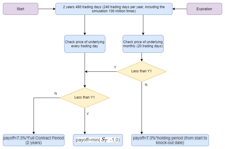
Pricing Workflow:

Assume there are 240 trading days per year, for a total of 480 trading days including the start date. Perform Monte Carlo simulation with 1,000,000 paths. First, generate a matrix z of size 1000000*480 filled with standard normally distributed random numbers.
Assume the initial stock price S0=1, volatility vol=13%, risk-free interest rate r=3%, and dividend yield q=8%. Use the random number matrix z to simulate stock price paths following the Geometric Brownian Motion.
Initialize s(：,1)=S0, and compute recursively s(：,i+1) = s(：,i) * exp((r-q-vol^2/2)*(1/240)+vol*sqrt(1/240)*z(：,i)).
For each of the 1,000,000 simulation paths:
- Daily knock-in observation: If the stock price falls below Y2=0.7, the option is considered knocked in.
- Monthly knock-out observation: Every 20 trading days, check whether the stock price exceeds Y1=1.0.
Based on the snowball option rules, there are three possible outcomes:
- If a knock-out event occurs on any observation day, the holder receives payoff=7.3%*holding period (from start to knock-out date).
- If the option neither knocks in nor knocks out during the 24-month period, the holder receives payoff=7.3%*Full Contract Period (2 years).
- If the option is knocked in at some point but not knocked out by maturity, the payoff is payoff=min( -1,0), where is the final price of the simulation path.
After 1,000,000 simulations, record the status, holding period, and payoff for each path. Then, discount each payoff to present value. The final snowball option price is the average of these discounted payoffs.
To ensure the accuracy of the computed price, calculate the option Greeks using the finite difference method, including Delta, Gamma, Theta, Vega, and Rho. Set to 0.005.
The formula for calculating Delta is , which means calculating the prices of snowball options with underlying prices , respectively.

The full implementation of this pricing algorithm is provided in Appendix.

3.2 Accelerating the Pricing Algorithm with Shark Graph

Appendix 1 presents a script that utilizes the ploop function to parallelize calculations and concatenate results on the CPU. In contrast, Appendix 2 demonstrates how the same workload can be accelerated using Shark Graph, which abstracts away the complexity of parallel programming by automatically optimizing operator execution on the GPU.

The following tests evaluated the performance of snowball option pricing using Shark Graph and DolphinDB’s CPU-based parallel programming.

The test environment was configured as follows:


Software/Hardware	Information
OS (Operating System)	CentOS Linux 7 (Core)
Kernel	3.10.0-1160.el7.x86_64
CPU Type	AMD EPYC 7513 32-Core Processor
Logical CPU Cores	128 cores
Memory	512 GB
GPU	NVIDIA A800 80GB PCIe

This case study measured the execution time (in milliseconds) of snowball option pricing under different levels of concurrency and Monte Carlo iteration counts, comparing CPU-based and GPU-accelerated calculations.

The results are summarized in the table below:


Concurrency	1K Iter	10K Iter	100K Iter	1M Iter
DolphinDB - 8	40.49	406.04	2,504.10	26,546.84
DolphinDB - 16	13.21	244.60	1,464.68	14,306.35
DolphinDB - 32	12.47	129.80	1,053.39	9,908.71
DolphinDB - 64	11.61	99.57	779.49	7,742.04
DolphinDB -128	27.38	63.39	577.26	6,213.23
Shark Graph	2.87	6.20	40.90	372.36

The acceleration ratios are shown in the Figure 2:

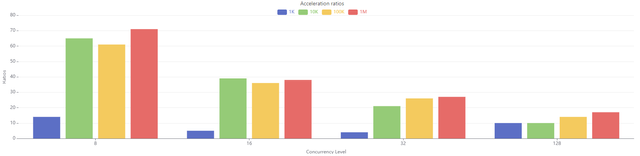
In large-scale simulations, Shark delivers a significant performance advantage over DolphinDB's CPU-based parallel execution. Compared to DolphinDB configured with 8 concurrent threads, Shark achieves up to a 70× acceleration. Even at moderate simulation scales, it consistently delivers over 60× acceleration. Although a single NVIDIA A800 GPU is approximately 9 to 10 times more expensive than a 32-core, 64-thread CPU, Shark outperforms DolphinDB running with 64 threads by a factor of 20×.

Therefore, for computation-intensive workloads, Shark's GPU acceleration providess a significantly more cost-effective solution.

4. Conclusion

This article presented a solution to accelerate DolphinDB scripts using the heterogeneous computing platform Shark. By simply annotating target functions with @gpu, users can seamlessly harness GPU acceleration with minimal code changes. In the snowball option pricing case, Shark delivered up to 65× acceleration compared to CPU-based concurrent execution. Even for moderately sized Monte Carlo simulations, Shark achieved a 57× performance improvement.

5. Appendix

Appendix 1: DolphinDB script for snowball option pricing

// % Number of simulation paths
N = 1000000;

// % Underlying asset parameters
vol   = 0.13;
S0    = 1;
r     = 0.03;
q     = 0.08;

// % Date parameters
days_in_year = 240; // trading days in a year
dt    = 1\days_in_year; // one trading day

// % Barrier option (embedded snowball) parameters
T     = 2; // term in years
Tdays = T * days_in_year; // term in trading days
Y1    = 1*S0;   // knock-out level
Y2    = 0.8*S0; // knock-in level
observation_idx = 20 + 20*(0..(Tdays/20 - 1)) // observation days for knock-out, observed only on these days
all_t = dt + dt*(0..(T * days_in_year - 1))

St = 1;

// % Target return rate
profit = 0.003 * S0;

con_level = 100

def coupon(N, vol, S0, r, q, T, Y1, Y2, observation_idx, St, profit, num){
	days_in_year = 240; // trading days in a year
	dt    = 1\days_in_year; // one trading day
	all_t = dt + dt*(0..int(T * days_in_year - 1))
	Tdays = int(T * days_in_year); // term in trading days

	S = St * exp((r - q - vol*vol/2) * repmat(matrix(all_t), 1, N) +
                 vol * sqrt(dt) * cumsum(norm(0,1,Tdays * N)$Tdays:N))

	// status
	knockout_matrix = S[observation_idx - 1, 0..(N - 1)] > Y1
	status = iif(sum(S[observation_idx - 1, 0..(N - 1)] > Y1) > 0, 1,
	             iif(sum(S < Y2) == 0, -1, 0))

	// t_holding (holding duration)
	k = observation_idx * (S[observation_idx - 1, 0..(N - 1)] > Y1)
	kk = iif(k == 0, NULL, k)
	kkk = bfill(kk)
	res = kkk[0,].flatten()
	t_holding = all_t[res].nullFill!(double(T))

	// pay_off
	tmp_nag = min(0, last(S)/S0 - 1)
	payoff = iif(status * t_holding > 0, status * t_holding,
	             iif(status * t_holding == 0, double(T), tmp_nag))

	res = table(status, t_holding, payoff)
	return res
}

def barrier_coupon(N, vol, S0, r, q, T, Y1, Y2, observation_idx, St, profit, con_level){
	con = int(N \ con_level)
	nloop = 1..(con_level)
	a = ploop(coupon{con, vol, S0, r, q, T, Y1, Y2, observation_idx, St, profit}, nloop).unionAll(false)

	if (- profit * N - (exec sum(exp(-r * t_holding) * payoff) from a where status = -1) > 0){
	    C = (- profit * N - (exec sum(exp(-r * t_holding) * payoff) from a where status = -1)) /
	        (exec sum(exp(-r * t_holding) * payoff) from a where status != -1)
	    return C
	}else{
		C = 0
	    return C
	} 
}

def pricing(N, vol, S0, r, q, T, Y1, Y2, observation_idx, St, profit, C, num){
	// % Date parameters
	days_in_year = 240; // trading days in a year
	dt    = 1\days_in_year; // one trading day
	all_t = dt + dt*(0..int(T * days_in_year - 1))
	Tdays = int(T * days_in_year); // term in trading days

	S = St * exp((r - q - vol*vol/2) * repmat(matrix(all_t), 1, N) +
                 vol * sqrt(dt) * cumsum(norm(0,1,Tdays * N)$Tdays:N))

	// status
	knockout_matrix = S[observation_idx - 1, 0..(N - 1)] > Y1
	status = iif(sum(S[observation_idx - 1, 0..(N - 1)] > Y1) > 0, 1,
	             iif(sum(S < Y2) == 0, -1, 0))

	// t_holding (holding duration)
	k = observation_idx * (S[observation_idx - 1, 0..(N - 1)] > Y1)
	kk = iif(k == 0, NULL, k)
	kkk = bfill(kk)
	res = kkk[0,].flatten()
	t_holding = all_t[res].nullFill!(double(T))

	// pay_off
	tmp_nag = min(0, last(S)/S0 - 1)
	payoff = iif(status * t_holding > 0, C * status * t_holding,
	             iif(status * t_holding == 0, C * double(T), tmp_nag))

	res = table(status, t_holding, payoff)
	return res
}

def barrier_pricing(N, vol, S0, r, q, T, Y1, Y2, observation_idx, St, profit, C, con_level){
	con = int(N \ con_level)
	nloop = 1..(con_level)
	a = ploop(pricing{con, vol, S0, r, q, T, Y1, Y2, observation_idx, St, profit, C}, nloop).unionAll(false)
	price = mean(exp(-r * a.t_holding) * a.payoff)
	return price
}

timer C = round(barrier_coupon(N, vol, S0, r, q, T, Y1, Y2, observation_idx, St, profit * S0, con_level), 3)

if (C > 0){
	timer price_St_plus  = barrier_pricing(N, vol, S0, r, q, T, Y1, Y2, observation_idx, St * (1 + 0.005), profit, C, con_level);
	timer price_St_minus = barrier_pricing(N, vol, S0, r, q, T, Y1, Y2, observation_idx, St * (1 - 0.005), profit, C, con_level);
	timer price_vol_plus = barrier_pricing(N, vol + 0.01, S0, r, q, T, Y1, Y2, observation_idx, St, profit, C, con_level);
	timer price_vol_minus = barrier_pricing(N, vol - 0.01, S0, r, q, T, Y1, Y2, observation_idx, St, profit, C, con_level);
	timer price_after_oneday = barrier_pricing(N, vol, S0, r, q, T - dt, Y1, Y2, observation_idx - 1, St, profit, C, con_level);
	timer price = barrier_pricing(N, vol, S0, r, q, T, Y1, Y2, observation_idx, St, profit, C, con_level);

	timer delta = (price_St_plus - price_St_minus) / 2 / St / (St * 0.005);
	timer gamma = (price_St_plus - 2 * price + price_St_minus) / St / St / (St * 0.005)^2;
	timer vega  = (price_vol_plus - price_vol_minus) / 2 / 0.01;
	timer theta = (price - price_after_oneday) / dt;
}
else {
	price = NULL
	delta = NULL
	gamma = NULL
	vega  = NULL
	theta = NULL
}

Appendix 2: Script for snowball option pricing using Shark Graph

// % Number of simulation paths
N = 1000000;

// % Underlying asset parameters
vol   = 0.13;
S0    = 1;
r     = 0.03;
q     = 0.08;

// % Date parameters
days_in_year = 240; // Trading days in one year
dt    = 1\days_in_year; // One trading day

// % Barrier option (embedded snowball) parameters
T     = 2; // Option term in years
Tdays = T * days_in_year; // Term in trading days
Y1    = 1 * S0;   // Knock-out price
Y2    = 0.8 * S0; // Knock-in price
observation_idx = 20 + 20 * (0..(Tdays / 20 - 1)) // Observation days (check knock-out only on these dates)
all_t = dt + dt * (0..(T * days_in_year - 1))

St = 1;

// % Target yield rate
profit = 0.003 * S0;

con_level = 100

def coupon(N, vol, S0, r, q, T, Y1, Y2, observation_idx, St, profit){

    days_in_year = 240; // Trading days in one year
    dt = 1\days_in_year; // One trading day
    all_t = dt + dt * (0..int(T * days_in_year - 1))
    Tdays = int(T * days_in_year); // Term in trading days

    S = St * exp((r - q - vol * vol / 2) * repmat(matrix(all_t), 1, N) +
                 vol * sqrt(dt) * cumsum(norm(0, 1, Tdays * N) $ Tdays:N))

    // Determine status
    knockout_matrix = S[observation_idx - 1, 0..(N - 1)] > Y1
    status = iif(sum(knockout_matrix) > 0, 1, iif(sum(S < Y2) == 0, -1, 0))

    // Holding period
    k = observation_idx * (knockout_matrix)
    kk = iif(k == 0, NULL, k)
    kkk = bfill(kk)
    res = kkk[0,].flatten()
    t_holding = all_t[res].nullFill(double(T))

    // Payoff
    statusxtholdings = status * t_holding
    tmp_nag = min(0, last(S)/S0 - 1)
    payoff = iif(statusxtholdings > 0, statusxtholdings,
                 iif(statusxtholdings == 0, double(T), tmp_nag))
    res = table(status, t_holding, payoff)

    index = res.status == -1
    aut = res.payoff[index]
    sum1 = sum(exp(-r * res.t_holding[index]) * res.payoff[index])

    if (-profit * N - sum1 > 0){
        index2 = res.status != -1
        sum2 = sum(exp(-r * res.t_holding[index2]) * res.payoff[index2])
        C = (-profit * N - sum1) / sum2
        return C
    } else {
        return 0
    }
}

// fn = createSharkGraph(snowRun)
// fn.genGraphDotFile("/home/jpma/testDB/release300.graph/build/dos/1.dot")
// fn.dumpGraphCode("/home/jpma/testDB/release300.graph/build/dos/D20-20840.rewrite.dos")

def pricing(N, vol, S0, r, q, T, Y1, Y2, observation_idx, St, profit, C, num){
    // % Date parameters
    days_in_year = 240; // Trading days in one year
    dt = 1\days_in_year; // One trading day
    all_t = dt + dt * (0..int(T * days_in_year - 1))
    Tdays = int(T * days_in_year); // Term in trading days

    S = St * exp((r - q - vol * vol / 2) * repmat(matrix(all_t), 1, N) +
                 vol * sqrt(dt) * cumsum(norm(0, 1, Tdays * N) $ Tdays:N))

    // Determine status
    knockout_matrix = S[observation_idx - 1, 0..(N - 1)] > Y1
    status = iif(sum(knockout_matrix) > 0, 1, iif(sum(S < Y2) == 0, -1, 0))

    // Holding period
    k = observation_idx * (knockout_matrix)
    kk = iif(k == 0, NULL, k)
    kkk = bfill(kk)
    res = kkk[0,].flatten()
    t_holding = all_t[res].nullFill(double(T))

    // Payoff
    statusxtholdings = status * t_holding
    tmp_nag = min(0, last(S)/S0 - 1)
    payoff = iif(statusxtholdings > 0, C * statusxtholdings,
                 iif(statusxtholdings == 0, C * double(T), tmp_nag))
    res = table(status, t_holding, payoff)
    return res
}

def barrier_pricing(N, vol, S0, r, q, T, Y1, Y2, observation_idx, St, profit, C){
    res = pricing(N, vol, S0, r, q, T, Y1, Y2, observation_idx, St, profit, C, 1)
    return mean(exp(-r * res.t_holding) * res.payoff)
}

@gpu
def snowRun(N, vol, S0, r, q, T, Y1, Y2, observation_idx, St, profit, con_level, dt) {
    C = round(coupon(N, vol, S0, r, q, T, Y1, Y2, observation_idx, St, profit * S0), 3) 
    if (C > 0) {
        price_St_plus = barrier_pricing(N, vol, S0, r, q, T, Y1, Y2, observation_idx, St * (1 + 0.005), profit, C);
        price_St_minus = barrier_pricing(N, vol, S0, r, q, T, Y1, Y2, observation_idx, St * (1 - 0.005), profit, C);
        price_vol_plus = barrier_pricing(N, vol + 0.01, S0, r, q, T, Y1, Y2, observation_idx, St, profit, C);
        price_vol_minus = barrier_pricing(N, vol - 0.01, S0, r, q, T, Y1, Y2, observation_idx, St, profit, C);
        price_after_oneday = barrier_pricing(N, vol, S0, r, q, T - dt, Y1, Y2, observation_idx - 1, St, profit, C);

        price = barrier_pricing(N, vol, S0, r, q, T, Y1, Y2, observation_idx, St, profit, C);
        delta = (price_St_plus - price_St_minus) / 2 / St / (St * 0.005);
        gamma = (price_St_plus - 2 * price + price_St_minus) / St / St / (St * 0.005)^2;
        vega = (price_vol_plus - price_vol_minus) / 2 / 0.01;
        theta = (price - price_after_oneday) / dt;
    } else {
        price = 1
        delta = NULL
        gamma = NULL
        vega = NULL
        theta = NULL
    }
    return price
}

timer {
    a1 = snowRun(N, vol, S0, r, q, T, Y1, Y2, observation_idx, St, profit, con_level, dt) 
}