
Calculate Stock Adjustment Factors and Adjusted Market Data
In quantitative trading, you often need to adjust historical stock market data to eliminate the impact of corporate actions, such as cash dividends, bonus shares, and stock splits, on price trends.
This tutorial is intended for quantitative beginners who are familiar with basic DolphinDB operations, including deployment, table creation, and code debugging. It explains how to calculate forward and backward adjustment factors from unadjusted daily stock OHLC data and generate the corresponding adjusted market data.
We explain the calculation logic using the "return-based adjustment" algorithm and implement it step by step in DolphinDB.
1. Unadjusted Market Data
Unadjusted market data refers to a stock's historical prices before any corporate-action adjustments. In this data, the closing price on each trading day directly reflects the actual market trading price.
Unadjusted data shows price jumps after corporate actions such as dividends, rights issues, or stock splits. For example, if a stock is priced at 10 yuan prior to the ex-rights date, its opening price on the ex-rights date drops sharply to 5 yuan due to a 10-for-10 stock split. If you plot an OHLC chart directly from unadjusted prices, the stock price appears to plunge by about 50% on the ex-rights date. This is not a real decline caused by changes in the company's fundamentals, but a nominal price change caused by the stock split.
Although unadjusted market data preserves the actual prices of all historical trades, it does not intuitively show the stock's true returns, and historical OHLC charts contain obvious gaps.
Common fields in unadjusted data include the trading date, stock code, opening price, closing price, highest price, lowest price, and previous closing price. For example:
trade_date ts_code open close pre_close ...
2008.06.12 600519.SH 157.48 151.21 157.49 ...
2008.06.13 600519.SH 148.11 149.49 151.21 ...
2008.06.16 600519.SH 147.70 144.50 148.65 ...
2008.06.17 600519.SH 143.51 141.97 144.50 ...
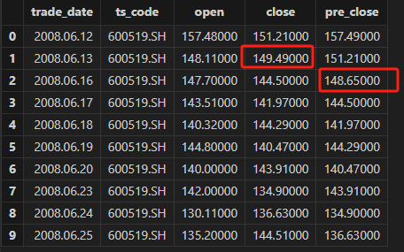
The table above shows a sample of unadjusted market data for Kweichow Moutai
(600519.SH) from June 12 to June 17, 2008. June 16, 2008 is the ex-rights date. In
the unadjusted data, pre_close (the previous closing price) jumps
on that date: pre_close on 2008.06.16 is 148.65, while
close on the previous trading day, 2008.06.13, is 149.49. This
jump creates a gap in the daily OHLC chart for 2008.06.16 relative to the previous
day.
If you calculate returns directly without applying price adjustments, the results can be misleading. For example, the unadjusted closing price of 144.50 on 2008.06.16 appears to be down 3.3% from the previous trading day's actual close of 149.49 ((144.5-149.49)\149.49). In fact, this change includes the effects of dividends and stock splits and does not represent an actual loss for investors who held the stock.
Price adjustment addresses such situation by correcting historical stock prices for corporate actions so that prices on different dates are comparable. After adjustment, the market data series before and after an ex-rights event can be joined smoothly, preserving the continuity of price trends and the accuracy of returns.
There are two main adjustment methods: backward adjustment, which keeps the initial price unchanged and adjusts future prices, and forward adjustment, which keeps the current price unchanged and adjusts historical prices. The following sections describe the calculation methods for backward adjustment and forward adjustment, and show how to use DolphinDB to calculate adjustment factors and generate adjusted market data.
2. Price Adjustments
Backward adjustment uses the price on the first listing day, or another selected base date, as the benchmark and adjusts subsequent stock prices. In simple terms, backward adjustment assumes that an investor has held one original share from the beginning and participated in all dividends and bonus share distributions, converting these corporate-action benefits into stock price appreciation. As a result, the current backward-adjusted price is higher than the actual price, reflecting the cumulative benefits from corporate actions.
Backward-adjusted market data makes it easy to see how much the stock price has cumulatively increased if it was bought at the beginning and held until the present. However, because actions such as rights issues may require additional capital, the return calculated from backward-adjusted prices is not necessarily the investor's actual return. It is only a theoretical measure of cumulative appreciation.
Forward adjustment uses the latest price as the benchmark and adjusts past historical prices. This approach preserves the actual level of recent prices and shifts pre-ex-rights prices downward so that the entire price series remains continuous.
2.1 Backward Adjustment
To generate backward-adjusted market data, you must first calculate the backward adjustment factor. The backward adjustment factor is a time-varying multiplier used to convert unadjusted prices to a level based on the initial price.
The return-based adjustment method defines the backward adjustment factor as follows:
Backward adjustment factor = forward cumulative product of (previous trading day's Close / current day's PrevClose)Here, "current day's previous closing price" refers to
pre_close in the unadjusted data. This value is usually
provided by the exchange and is already adjusted for corporate actions on
ex-rights/ex-dividend dates.
According to this formula:
- If no corporate action occurs on the day, the current day's previous closing price equals the previous day's closing price. The backward adjustment factor is previous day's closing price ÷ current day's previous closing price = 1, so the factor remains unchanged.
- If the day is an ex-rights/ex-dividend date, the current day's previous closing price has been adjusted for corporate actions and differs from the previous day's actual closing price. The backward adjustment factor equals the previous trading day's close divided by the current day's previous closing price, and is greater than 1.
The backward adjustment factor is defined as 1 on the first listing day. When no corporate action occurs, the factor remains unchanged. Each time an ex-rights/ex-dividend event occurs, the factor is multiplied by the ratio described above. This means the backward adjustment factor is the cumulative product of all historical corporate-action ratios, and it is ultimately used to scale up unadjusted prices.
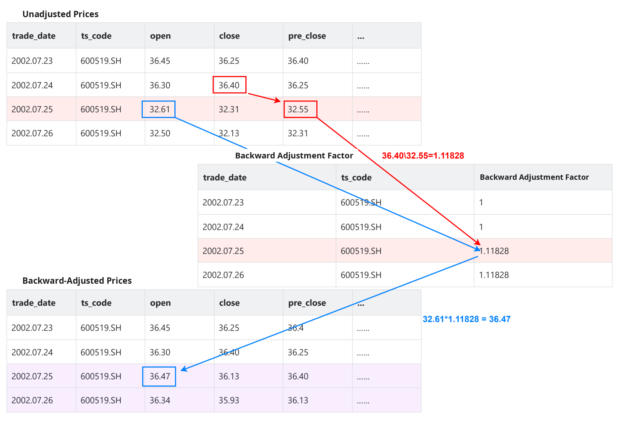
As shown in the preceding figure, Kweichow Moutai (600519.SH) carried out its first corporate action on 2002.07.25: 1 bonus share from capital reserves for every 10 shares and a cash dividend of 6 yuan per 10 shares, including tax.
- In the unadjusted market data, 2002.07.25 is the first ex-rights date. The current day's previous closing price drops from 36.40 to 32.55, as highlighted by the red box.
- Using the formula, the backward adjustment factor is 1.11828 (36.40\32.55).
- Backward-adjusted market data is calculated by multiplying all price-related
fields in the unadjusted market data by the backward adjustment factor. The
figure uses the opening price
openas an example to illustrate the calculation logic.
By cumulatively multiplying the backward adjustment factors, we convert all historical prices to a level based on the initial price. Backward-adjusted market data can be obtained by multiplying unadjusted market data by the backward adjustment factor for the corresponding date.
2.2 Forward Adjustment
Similarly, to generate forward-adjusted market data, you must first calculate the forward adjustment factor. The forward adjustment factor is used to scale down historical unadjusted prices by a certain ratio.
According to the return-based adjustment algorithm, the forward adjustment factor is defined as follows:
Forward adjustment factor = reverse cumulative product of (current day's PrevClose / previous trading day's Close)It has a reciprocal scaling relationship with the backward adjustment factor. When a corporate action occurs, the unadjusted previous closing price decreases, causing the forward adjustment factor to be less than 1. When no corporate action occurs, the current day's previous close equals the previous day's close, so the forward adjustment factor is 1.
The forward adjustment factor is reset to 1 on the first trading day after the most recent ex-rights/ex-dividend date. In other words, each time a new corporate-action event occurs, the forward adjustment factor jumps to a smaller value, because the current day's adjusted previous closing price is lower than the previous day's actual closing price.
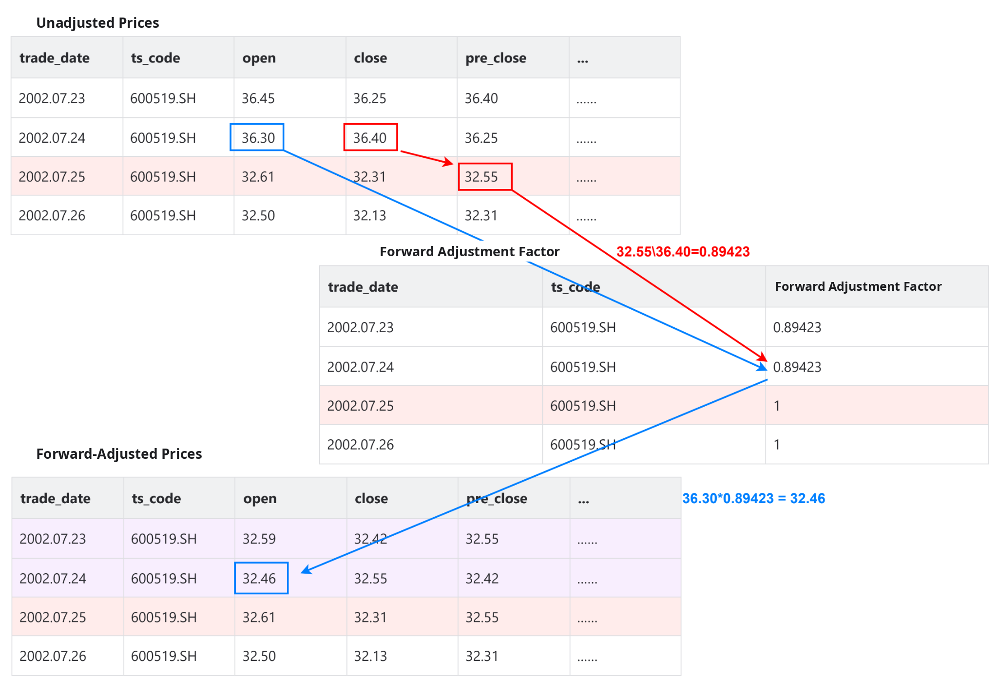
As shown in the preceding figure, Kweichow Moutai (600519.SH) carried out its first corporate action on 2002.07.25: 1 additional share converted from capital reserve for every 10 shares and a cash dividend of 6 yuan per 10 shares, tax included.
- In the unadjusted market data, 2002.07.25 is the first ex-rights date. The previous closing price for that day drops from 36.40 to 32.55, as highlighted by the red box.
- Using the formula, the forward adjustment factor is 0.89423 (32.55\36.40).
- Forward-adjusted market data is calculated by multiplying all price-related
fields in the unadjusted market data by the forward adjustment factor. The
figure uses the opening price,
open, to illustrate the calculation logic.
In summary, the forward adjustment factor adjusts historical stock prices to the same baseline as the current price by successively multiplying unadjusted prices by these factors, which are less than 1.
3. Code Implementation
3.1 Store Unadjusted Market Data
This section uses the unadjusted CSV market data in the appendix as an example. This data is typically provided by the exchange, and on ex-rights dates, the previous closing price for that day is adjusted based on the rights and dividend information.
Create the database and partitioned table:
if(not existsDatabase("dfs://stock_day_k")){
    create database "dfs://stock_day_k"
    partitioned by VALUE(2025.01M..2025.05M),
    engine="OLAP"
}else{
    print("The database has created.")
}

create table "dfs://stock_day_k"."stock_day_k"(
    trade_date  DATE[comment="Trading date"],
    ts_code     SYMBOL[comment="Stock code"],
    open        DOUBLE[comment="Opening price"],
    high        DOUBLE[comment="Highest price"],
    low         DOUBLE[comment="Lowest price"],
    close       DOUBLE[comment="Closing price"],
    pre_close   DOUBLE[comment="Previous closing price"],
    vol         DOUBLE[comment="Trading volume"],
    amount      DOUBLE[comment="Trading value"]
)
partitioned by trade_date
Import the unadjusted CSV market data. Modify the CSV file path according to your environment:
csvPath = "/hdd/hdd2/tutorial/stock_adj/600519.csv"
data = loadText(csvPath)
loadTable("dfs://stock_day_k", "stock_day_k").append!(data)
View a segment of the unadjusted market data for Kweichow Moutai (600519.SH) from June 12 to June 17, 2008:
stock_day_k = loadTable("dfs://stock_day_k", "stock_day_k")

select
 top 10 trade_date,ts_code,open,close,pre_close
from stock_day_k
where ts_code="600519.SH", trade_date>=2008.06.12
Output:
3.2 Calculate and Store Backward-Adjusted Data
Create the database and partitioned table for storing backward adjustment factors and market data:
if(not existsDatabase("dfs://stock_back")){
    create database "dfs://stock_back"
    partitioned by VALUE(2025.01M..2025.05M),
    engine="OLAP"
}else{
    print("The database has created.")
}

create table "dfs://stock_back"."stock_back"(
    trade_date  DATE[comment="Trading date"],
    ts_code     SYMBOL[comment="Stock code"],
    open        DOUBLE[comment="Opening price"],
    high        DOUBLE[comment="Highest price"],
    low         DOUBLE[comment="Lowest price"],
    close       DOUBLE[comment="Closing price"],
    pre_close   DOUBLE[comment="Previous closing price"],
    vol         DOUBLE[comment="Trading volume"],
    amount      DOUBLE[comment="Trading value"],
    adj_back    DOUBLE[comment="Backward adjustment factor"]
)
partitioned by trade_date
Calculate the backward adjustment factors and backward-adjusted market data from the unadjusted market data according to the formulas, and write the results to the corresponding database tables:
//Calculate backward adjustment factors
def calOneCodeFunc(code){
    /*@test
    code = "600519.SH"
    */
    //Load the daily unadjusted price data for one stock into memory
    one_code_data =
        select *
        from loadTable("dfs://stock_day_k", "stock_day_k")
        where ts_code=code
    //Handle the closing price when close is NULL on a suspended trading day
    update one_code_data
    set fill_close=iif(close==NULL and pre_close==prev(close),
                        prev(close),
                        iif(close==NULL,pre_close,close))
    //Calculate backward adjustment factors
    update one_code_data
    set adj_back=iif(cumcount(fill_close)==1, 1, cumprod(prev(fill_close)\pre_close))
    //Table containing adjustment factors and adjusted price data
    result =
        select
            trade_date,
            ts_code,
            open*adj_back as open,
            high*adj_back as high,
            low*adj_back as low,
            close*adj_back as close,
            pre_close*adj_back as pre_close,
            vol,
            amount,
            adj_back
        from one_code_data
    return result
}
//Process all stocks in the unadjusted price table
calCodes = exec distinct ts_code from loadTable("dfs://stock_day_k", "stock_day_k")
//Calculate in parallel by stock code
stock_back = ploop(calOneCodeFunc, calCodes).unionAll()
//Write to the backward-adjusted partitioned table
loadTable("dfs://stock_back", "stock_back").append!(stock_back)
Query data for key ex-rights dates:
select *
from loadTable("dfs://stock_back", "stock_back")
where ts_code="600519.SH", trade_date in [2002.07.25,2003.07.14,2004.07.01]
Output:

3.3 Calculate and Store Forward-Adjusted Data
Create the database and partitioned table for storing forward adjustment factors and market data:
if(not existsDatabase("dfs://stock_pre")){
    create database "dfs://stock_pre"
    partitioned by VALUE(2025.01M..2025.05M),
    engine="OLAP"
}else{
    print("The database has created.")
}

create table "dfs://stock_pre"."stock_pre"(
    trade_date  DATE[comment="Trading date"],
    ts_code     SYMBOL[comment="Stock code"],
    open        DOUBLE[comment="Opening price"],
    high        DOUBLE[comment="Highest price"],
    low         DOUBLE[comment="Lowest price"],
    close       DOUBLE[comment="Closing price"],
    pre_close   DOUBLE[comment="Previous closing price"],
    vol         DOUBLE[comment="Trading volume"],
    amount      DOUBLE[comment="Trading value"],
    adj_pre   DOUBLE[comment="Forward adjustment factor"]
)
partitioned by trade_date
Calculate the forward adjustment factors and forward-adjusted market data from the unadjusted market data according to the formulas, and write the results to the corresponding database tables:
def calOneCodeFunc(code){
    /*@test
    code = "600519.SH"
    */
    //Load the daily unadjusted price data for one stock into memory
    one_code_data =
        select *
        from loadTable("dfs://stock_day_k", "stock_day_k")
        where ts_code=code
    //Handle the closing price when close is NULL on a suspended trading day
    update one_code_data
    set fill_close=iif(close==NULL and pre_close==prev(close),
                        prev(close),
                        iif(close==NULL,pre_close,close))
    //Calculate backward adjustment factors
    update one_code_data
    set adj_back=iif(cumcount(fill_close)==1, 1, cumprod(prev(fill_close)\pre_close))
    //Calculate forward adjustment factors
    update one_code_data
    set adj_pre=adj_back/last(adj_back)
    //Table containing adjustment factors and adjusted price data
    result =
        select
            trade_date,
            ts_code,
            open*adj_pre as open,
            high*adj_pre as high,
            low*adj_pre as low,
            close*adj_pre as close,
            pre_close*adj_pre as pre_close,
            vol,
            amount,
            adj_pre
        from one_code_data
    return result
}
//Process all stocks in the unadjusted price table
calCodes = exec distinct ts_code from loadTable("dfs://stock_day_k", "stock_day_k")
//Calculate in parallel by stock code
stock_pre = ploop(calOneCodeFunc, calCodes).unionAll()
//Write to the forward-adjusted partitioned table
loadTable("dfs://stock_pre", "stock_pre").append!(stock_pre)
Query data for key ex-rights dates:
select *
from loadTable("dfs://stock_pre", "stock_pre")
where ts_code="600519.SH", trade_date in [2002.07.25,2003.07.14,2004.07.01]
Output:

4. Frequently Asked Questions (FAQ)
4.1 Incorrect Adjustment Factor Calculation Results
Possible causes:
- The unadjusted market data is incomplete, especially the data during suspended trading periods. You can use the Kweichow Moutai data provided in the appendix as a baseline and compare it with the stock data in your database to verify completeness. Pay special attention to whether the data values from 2006.05.19 to 2006.05.24 are consistent.
- The unadjusted market data is incorrect. You can cross-check it against the sample data in the appendix.
Resolution: Complete the missing data and ensure the quality of the unadjusted market data.
4.2 Differences from Third-Party Data Vendors
Possible causes:
- Decimal precision.
- Differences in adjustment calculation methods.
Resolution: While ensuring the quality of the unadjusted data, derive results from the actual data, analyze the causes of the differences in detail, and then decide how to proceed.
5. Appendix
- Unadjusted market data: 600519.csv
- Backward-adjusted market data: 600519_back.csv
- Forward-adjusted market data: 600519_pre.csv
- Tutorial code: stock_adj.dos