
Factor Attribution Analysis Based on DolphinDB
In financial markets, every stock is exposed to multiple factors at any given point in time, and the combined effects of these factors drive fluctuations in stock prices. With the widespread adoption of quantitative methods and big data technologies, more investors are using multi-factor models to explain and forecast stock returns. These factors include style factors (e.g., momentum, value, volatility, and size), industry factors, and specific factors. Together, they reveal the sources of systematic changes in stock prices from different perspectives.
Factor attribution analysis systematically decomposes a portfolio's excess returns and active risk relative to a benchmark into different risk factors, helping identify and quantify each factor's contribution to portfolio performance. This analysis not only helps evaluate a portfolio's historical performance but also serves as an important reference for future portfolio optimization and risk control. The overall factor attribution workflow consists of three parts: pure factor return estimation, active return attribution, and active risk attribution. This article introduces a factor attribution module implemented in DolphinDB based on the factor attribution model, enabling you to perform factor attribution analysis.
1. Model Introduction
A multi-factor model is a financial model used to explain and forecast stock returns. It assumes that portfolio returns are jointly determined by multiple factors. We first provide a brief introduction to the multi-factor model in Barra CNE5+. Assume a portfolio of N stocks. For any stock j, its excess return is linearly decomposed into K factors, including p industry factors and q style factors. The general expression is as follows:

where rj is the excess return of stock j, Xi represents the exposure vector of factor i, fi is the factor return vector of factor i, and μⱼ is the active residual of stock j. Let X = [X1, X2, …, XK] denote the factor exposure matrix, and let r = [r₁, r₂, ..., rN] denote the vector of excess returns of N stocks on day T.
-
The factor exposure matrix X consists of a dummy industry factor matrix and a risk factor exposure matrix. The dummy industry factor matrix is generated from each stock's industry classification, and the risk factor exposure matrix is derived from the stock's historical data over T days.
The pure factor return fi is calculated from the pure factor portfolio weights ωi and the stock excess return vector r, as follows:

The following sections describe the three main steps of factor attribution: pure factor return estimation, active return attribution, and active risk attribution.
1.1 Pure Factor Return Estimation
A pure factor stock portfolio is designed to be exposed only to a specific factor while remaining neutral to other style factors and industry factors, making it easier to analyze the factor's actual return and risk characteristics. Therefore, we need to estimate the pure factor portfolio weights for each style factor under industry-neutral and style-neutral constraints. Industry neutrality means the portfolio's industry allocation is consistent with the benchmark's, while style neutrality means the portfolio has zero risk exposure to style factors relative to the benchmark.
Based on the pure factor stock portfolio described above, consider the j-th style factor. The linear programming problem is formulated as follows:
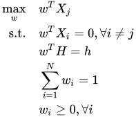
Objective function: ω is the weight vector of the j-th style factor, and Xj is the exposure vector of the j-th style factor. The factor attribution module maximizes the target factor exposure. Other common objective functions include maximizing the portfolio's Sharpe ratio and minimizing portfolio risk.
Constraints: The first constraint enforces style neutrality, ensuring zero exposure to the remaining style factors. The second constraint enforces industry neutrality, where H is the dummy industry factor matrix for the stocks and h is the benchmark's industry weight vector. Because short operations are not allowed in the Chinese A-share market, each stock weight must be constrained to be non-negative.
Note that the constraints above only ensure zero exposure to the remaining style factors; they do not strictly constrain exposure to the specified factor to one unit. The factor attribution module adds the following constraint:

Therefore, under industry-neutral and style-neutral constraints, pure factor portfolio weights ωj with full exposure to different style factors j are constructed and combined with the T-day stock excess return vector r to obtain the pure factor returns:

1.2 Active Return Attribution
Active return attribution systematically decomposes a stock portfolio's excess return (portfolio return minus benchmark return) into different factors, helping investors identify the sources of excess returns and evaluate the effectiveness and rationale of each factor. Because industry factors are neutralized when constructing pure factor portfolios, attribution analysis is performed only on the q style factors. The active return attribution model is as follows:
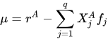
Let the stock portfolio weights and benchmark weights be ωP and ωb, respectively. The active weight is then ωA = ωP - ωb. Based on the style factor exposure matrix X and the excess return vector r, calculate the factor-wise active exposure XA = ωA·X and the excess return value rA = ωA·r. Combined with the pure factor return vector f = [f1, f2, ⋯, fq] obtained in Section 1.1, the portfolio's excess return can be decomposed as follows:
Factor contribution = XAf
Residual:
1.3 Active Risk Attribution
Active risk attribution decomposes a stock portfolio's risk relative to the benchmark into different factors. This helps investors identify excessive concentration or excessive deviation from a particular factor and better control the sources of risk in investment decisions. Based on the X-Sigma-Rho attribution model proposed by MSCI Barra, the expression for active risk attribution is:

where XA is the factor-wise active exposure, σ is the variance of volatility, and ρ is the correlation. As shown in the expression above, the active risk of stock portfolio return rA is attributed to factor-wise active exposure, factor return volatility, and correlation. Factor-wise active exposure reflects the portfolio's style tilt and is the primary source of the active risk. Factor return volatility reflects passive sources of risk that the portfolio cannot control. The correlation reflects the co-movement between stock portfolio returns and factors.
2. Module Usage
2.1 Data Preprocessing
First, create the data tables required for factor attribution to ensure that their fields match the examples below. If you do not have the required data tables, refer to Appendix 2 to generate simulated data. Partial simulated data are shown below:
-
Market benchmark information (bench): daily benchmark weights for individual stocks.
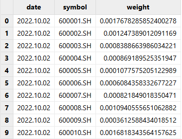
Figure 1. Figure 2-1 Market Benchmark Information Table -
Position weight table (own): daily position weights for individual stocks.
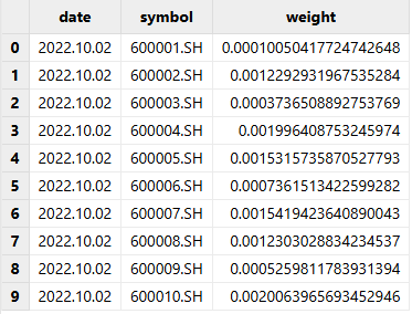
Figure 2. Figure 2-2 Position Weight Table -
Stock return table (market): daily returns for individual stocks.
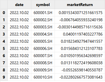
Figure 3. Figure 2-3 Stock Return Table -
Style factor exposure table (styleExpos): daily style factor exposures for individual stocks.

Figure 4. Figure 2-4 Style Factor Exposure Table -
Industry factor exposure table (industryExpos): daily dummy industry factor variables for individual stocks.
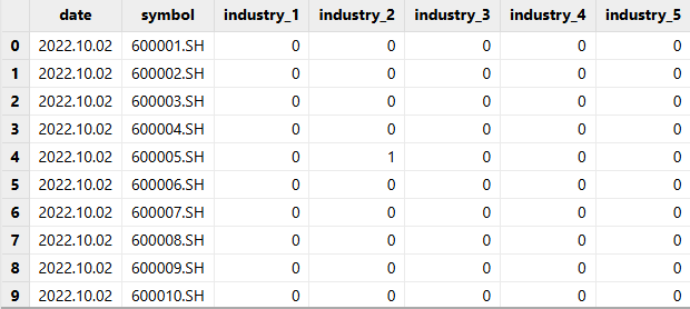
Figure 5. Figure 2-5 Industry Factor Exposure Table
2.2 Parameter Settings
In addition to the data tables required for factor attribution, you must set startDate and endDate to define the attribution analysis period. To standardize the style factor exposure table, set standard=true.
2.3 Function Calls
Use getHomeDir() to obtain the home directory, and place the
module file from Appendix 1 in the corresponding module path. Import the factor
attribution module with use:
use factorAttributionUtils
go
After setting the required parameters, call the function to obtain the attribution results: the pure factor return table (purefactorTb), the factor contribution residual table (factorAttResTb), and the active risk attribution table (riskTb).
attriResultDict = attributionFunc(startDate, endDate, bench, own, market, styleExpos,
 industryExpos, windowSize, standard=false)
2.4 Result Check
Specify a key of attriResultDict(pure_factor_returns, active_return_attribution, or active_risk_attribution) to retrieve the corresponding attribution table, for example, attriResultDict[`pure_factor_returns]. The results for the simulated data are as follows:



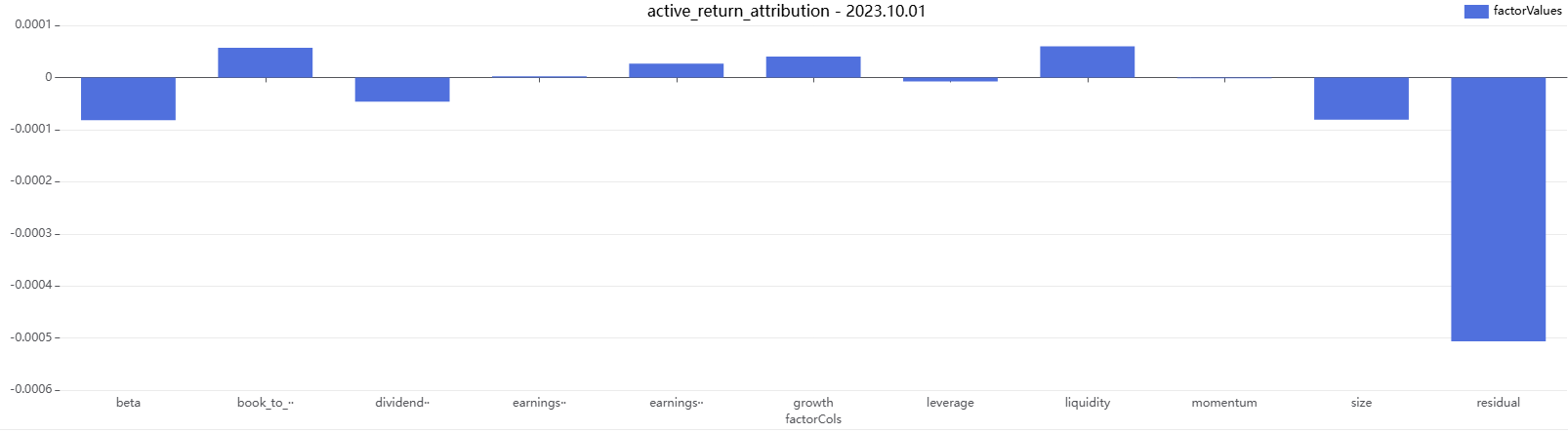
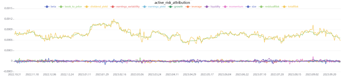
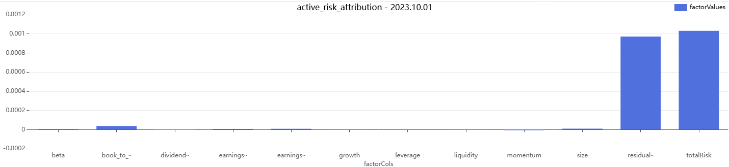
To visualize the results, specify resType and targetDate:
resType = "pure_factor_returns" //Specify "pure_factor_returns", "active_return_attribution", or "active_risk_attribution"
resTb = attriResultDict[resType]
factorCols = columnNames(resTb)[1:]
plot(resTb[factorCols], resTb[`date], resType)
//To view factor attribution results for a specific day, specify targetDate
targetDate = 2023.10.01
sliceData = select * from resTb where date = targetDate
factorValues = flatten(matrix(sliceData[factorCols]))
plot(factorValues, factorCols, resType+" - " + string(targetDate), COLUMN)
The results for the simulated data are plotted below. The following figures show sample result curves for selected factor attributions:
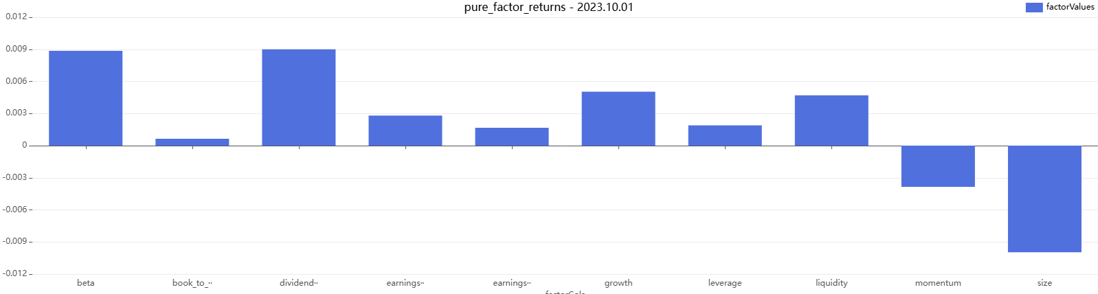
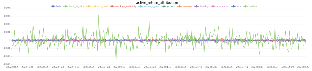
3. Function Performance
The functions in the factor attribution module use DolphinDB's built-in functions peach and each to perform concurrent computation across different trading days and style factors, improving the efficiency of factor attribution calculations. This section demonstrates the computational performance of the attribution function attributionFunc based on DolphinDB. Performance tests with different date ranges (startDate and endDate) and windowSize settings help you better understand the computational complexity of the module functions and their performance in practical applications.
3.1 Test Method
Simulated Data:
-
Benchmark data (bench): Simulates daily benchmark positions over 10 years.
-
Holding weight data (own): Simulates daily position weights over 10 years.
-
Return data (market): Simulates return data for 1,000 stocks over 10 years.
-
Style factor exposures (styleExpos): Simulates exposure information for 10 style factors over 10 years.
-
Industry factor exposures (industryExpos): Simulates exposure information for 30 industry factors over 10 years.
3.2 Test Results
The tests use different backtesting periods and numbers of style factors. With daily rebalancing, the elapsed time for running the attribution function is as follows:
Table 3-1 Test Results
| Backtesting Period | Number of Style Factors | Elapsed Time |
|---|---|---|
| 10 years | 20 | 1 min 43s |
| 5 years | 20 | 48s |
| 1 year | 20 | 11s |
| 10 years | 10 | 32s |
| 5 years | 10 | 17s |
| 1 Year | 10 | 3s |
4. Summary
This article describes the implementation of an attribution module based on the factor attribution model, using DolphinDB's built-in statistical analytic function library, efficient parallel computing, convenient table joins, and vectorized programming. By combining DolphinDB's powerful computing capabilities with the factor attribution model, you can perform attribution analysis more efficiently and accurately, and understand the sources of portfolio excess returns and risk, which is an essential part of investment decision-making.
5. Appendix
-
Module file: factorAttributionUtils.dos
-
Module test file: factorTestScript.dos
-
Detailed function description: factor_attribution_parameter_description.pdf