
Synthesize OHLC Bars and Continuous Contracts from Snapshot Data
Due to differences in trading hours across futures instruments and varying levels of activity among contracts, synthesizing minute-level OHLC bars from snapshot market data requires different approaches to time alignment depending on the scenario.
To address this, we have developed the FuturesOLHC module, which encapsulates the above processing logic. By simply calling the functions defined in the module, you can easily achieve the following:
-
Synthesize minute-level OHLC bars from historical futures snapshot market data
-
Synthesize continuous contract market data from historical futures snapshot market data
-
Synthesize minute-level OHLC bars from real-time futures snapshot market data
This tutorial walks you through the following:
-
First, it details how to synthesize minute-level OHLC bars from historical futures snapshot market data;
-
Next, it explains how to synthesize continuous contract market data from historical futures snapshot market data;
-
Then, it describes how to synthesize minute-level OHLC bars from real-time futures snapshot market data;
-
Finally, it introduces the structure and functionality of the
FuturesOLHCmodule and provides examples of implementing the above three scenarios using the functions defined in the module.
This tutorial applies to multiple exchanges, including: China Financial Futures Exchange, Dalian Commodity Exchange, Shanghai Futures Exchange, Shanghai International Energy Exchange, Zhengzhou Commodity Exchange, and Guangzhou Futures Exchange.
Note: All code in this article must run on DolphinDB server version 2.00.14 or later.
1. Synthesize Minute-Level OHLC Bars from Historical Snapshot Market Data
1.1 Characteristics of Futures Snapshot Data
Tick-by-tick data is the most granular and comprehensive record of market activity, capturing every market event — including each trade execution and every new order submission. As it logs data at the level of each discrete market event, tick data is regarded as the most precise form of market data available. In contrast, snapshot data is a sample statistic derived from tick data. In other words, it is the statistical result of slicing market information at a certain frequency along the time dimension. If market information is considered a time-series data stream, snapshot data is equivalent to periodically capturing this data stream to show the market state at a given moment, while tick data is the complete record of the data stream. Consequently, tick data offers superior precision, while the precision of snapshot data is inherently dependent on the sampling interval.
In the Chinese futures market, snapshot market data is sampled at 500 ms (i.e., one push every 0.5 seconds), but the push frequency is not strictly uniform. Different data vendors and exchanges may provide different snapshot market data fields, so even with a 500 ms sampling frequency, the specific fields and data formats may vary.
This tutorial standardizes the processing of futures data. The common fields in the futures snapshot market data table are as follows:
| Field name | Data type | Description |
|---|---|---|
| SortCo | SYMBOL | Exchange code |
| InstruID | SYMBOL | Futures contract code |
| TradeDay | DATE | Trading day |
| ClearingDay | DATE | Settlement date |
| TradeTime | TIME | Trade time |
| LastPrice | DOUBLE | Last price |
| PreSetPrice | DOUBLE | Previous settlement price |
| PreCloPrice | DOUBLE | Previous closing price |
| OpenPrice | DOUBLE | Opening price |
| HighPrice | DOUBLE | High price |
| LowPrice | DOUBLE | Low price |
| Volume | INT | Trading volume |
| Turnover | DOUBLE | Trading value (Turnover) |
| OpenInt | INT | Open interest |
| SetPrice | DOUBLE | Settlement price |
| ULimitPrice | DOUBLE | Limit up price of the day |
| LLimitPrice | DOUBLE | Limit down price of the day |
| ...... | ...... | The snapshot market data contains a large number of fields; for the complete field list, refer to the Appendix. |
The key fields involved in minute-bar calculation are as follows:
| Field name | Data type | Description |
|---|---|---|
| LastPrice | DOUBLE | Last price |
| PreSetPrice | DOUBLE | Previous settlement price |
| PreCloPrice | DOUBLE | Previous closing price |
| OpenPrice | DOUBLE | Opening price |
| HighPrice | DOUBLE | High price |
| LowPrice | DOUBLE | Low price |
| Volume | INT | Trading volume |
| Turnover | DOUBLE | Trading value (Turnover) |
| OpenInt | INT | Open interest |
| SetPrice | DOUBLE | Settlement price |
| ULimitPrice | DOUBLE | Limit up price of the day |
| LLimitPrice | DOUBLE | Limit down price of the day |
Based on the above fields, the minute-level OHLC bar indicators and calculation rules synthesized from futures snapshot market data are as follows (the calculation window is left-open, right-closed):
| Field name | Data type | Description | Calculation Rule |
|---|---|---|---|
| OpenPrice | DOUBLE | Opening price |
The latest price of the first snapshot market data within the calculation window
|
| HighPrice | DOUBLE | High price |
The highest price within the calculation window
|
| LowPrice | DOUBLE | Low price |
The lowest price within the calculation window
|
| ClosePrice | DOUBLE | Closing price |
The latest price of the last snapshot market data within the calculation window
|
| Volume | LONG | Trading volume | Sum of trading volumes of all snapshot market data within the calculation window; if snapshot data is missing, fill with 0. |
| Value | DOUBLE | Trading value |
Sum of trading values of all snapshot market data within the calculation window If snapshot data is missing, fill with 0. |
| Vwap | DOUBLE | Volume-weighted average price (VWAP) | Trading value/trading volume within the calculation window. |
| OpenInt | INT | Open interest | Current open interest |
| PreSetPrice | DOUBLE | Yesterday's settlement price | Yesterday's settlement price |
| SetPrice | DOUBLE | Settlement price | Today's settlement price, calculated based on minute closing prices during the day's trading. |
| ULimitPrice | DOUBLE | Limit up price | The limit up price from the day's snapshot market data. If the snapshot market data is missing within the intraday calculation window, populate it with the limit up price of the previous OHLC bar. |
| LLimitPrice | DOUBLE | Limit down price | The limit down price from the day's snapshot market data. If the snapshot market data is missing within the intraday calculation window, populate it with the limit down price of the previous OHLC bar. |
| PreClosePrice | DOUBLE | Previous closing price | The previous closing price from the day's snapshot market data. If the snapshot market data is missing within the intraday calculation window, populate it with the previous closing price of the previous OHLC bar. |
1.2 Rules for Synthesizing Snapshot Data
1.2.1 Handle High and Low Prices
Snapshot market data are time-interval data slices. The high and low prices in snapshot market data reflect the highest and lowest prices from the market open to the current snapshot timestamp, rather than the high and low within the snapshot interval. However, the high and low prices in an OHLC bar are the highest and lowest prices within the calculation window. Therefore, the high and low of a bar cannot be synthesized simply from the high and low prices in snapshot market data.
If the high (low) price in the snapshot data within the bar window is higher (lower) than the high (low) price in the snapshot data preceding the bar window, then the high (low) price in the snapshot data within the window is the bar's high (low). For example, if the last prices of the snapshots within the window are [3.0, 3.0, 3.11, 3.10], the high prices are [3.12, 3.12, 3.12, 3.12], and the high price of the snapshot immediately preceding the window is 3.11, then the high of the bar is 3.12. If the high price of the snapshot immediately preceding the window is 3.12, the bar's high (low) is calculated as follows: consistent with common industry practice, we use the maximum (minimum) of the last price within the window as the bar's high (low). The user-defined calculation function for the high price of a minute-level OHLC bar is as follows:
defg high(deltasHighPrice, highPrice, lastPrice){
	if(sum(deltasHighPrice)>0.000001){
		return max(highPrice)
	}
	else{
		return max(lastPrice)
	}
}
Parameter Description:
-
deltasHighPrice: The difference between the day's high prices (highPrice) of two consecutive snapshot slices for the same futures contract. A value greater than 0 indicates that the intraday high occurred within this interval, in which case the interval's high price is this value (highPrice).
-
highPrice: The day's high price from the snapshot market data.
-
lastPrice: The last price from the snapshot market data.
Note that this is an approximation algorithm. The last price (lastPrice) of each snapshot within the calculation window may not fully capture the true high and low over the entire window. For example, in the case above, the high price of the snapshot immediately preceding the bar window is 3.12. According to the algorithm, the bar's high is the maximum lastPrice within the window, which is 3.11. However, in practice, a trade at 3.12 may well have occurred within the window. To obtain the true high and low prices of an OHLC bar, tick-by-tick trade data must be used instead of snapshot data.
Similarly, the user-defined function for calculating the low price of a minute-level OHLC bar is as follows:
defg low(deltasLowPrice, lowPrice, lastPrice){
	sumDeltas = sum(deltasLowPrice)
	if(sumDeltas<-0.000001 and sumDeltas!=NULL){
		return min(iif(lowPrice==0.0, NULL, lowPrice))
	}
	else{
		return min(lastPrice)
	}
}
Parameter Description:
-
deltasLowPrice: The difference between the daily low prices (lowPrice) of two consecutive snapshot slices for the same futures contract. A value less than 0 indicates that the intraday low occurred within this interval, in which case the interval's low price is this value (lowPrice).
-
lowPrice: The daily low price from the snapshot market data.
-
lastPrice: The last price from the snapshot market data.
1.2.2 Handle Trading Volume, Trading Value, and Number of Trades
The trading volume, trading value, and number of trades in snapshot market data are all cumulative daily totals. Therefore, before performing rolling window calculations, the incremental difference between two consecutive snapshots must be derived first. The built-in deltas function and context by SQL clause in DolphinDB are used for data preprocessing. The specific implementation will be described in detail below.
1.2.3 No Trades After Market Open
For some thinly traded futures contracts, no trades may occur after trading begins at 09:00:00, although snapshot data continues to be pushed normally.
For calculation windows where no trades have occurred since the market open, this tutorial applies the following rules:
-
OpenPrice, HighPrice, LowPrice, ClosePrice, Volume, Value are set to 0.
-
PreClosePrice, ULimitPrice, LLimitPrice are set to the corresponding values from the snapshot market data.
1.2.4 No Trades Within an Intraday Calculation Window
For some thinly traded futures contracts, certain intraday calculation windows may contain no trades at all, although snapshot data continues to be pushed normally.
For calculation windows with no intraday trades, this tutorial applies the following rules:
-
OpenPrice, HighPrice, LowPrice, ClosePrice are set to the ClosePrice of the previous OHLC bar
-
Volume, Value are set to 0
-
PreClosePrice, ULimitPrice, LLimitPrice are set to the corresponding values of the previous OHLC bar
1.3 Steps for Calculating Minute-Level OHLC Bars
The following sections detail the steps for calculating minute-level OHLC bars from historical futures snapshot data as implemented in the module in the appendix.
1.3.1 Generate a Minute-Level OHLC Bar Alignment Table for Different Futures Products
Since trading hours vary across futures instruments, a minute bar alignment table is generated based on the trading sessions and contract codes of each futures instrument. The table contains the complete set of valid trading minutes for each futures instrument and is used to align minute bars.
For example, the SSE 50 Index, CSI 300 Index, CSI 500 Index, and CSI 1000 Index futures trade from 9:30 to 11:30 and from 13:00 to 15:15. To calculate 1-minute-level OHLC bars, the table includes data for each minute within the two trading sessions (9:30-11:30 and 13:00-15:15) for these index futures.
Note:
For detailed steps on generating the alignment table, refer to the appendix.
1.3.2 Define the Function for Calculating Minute-Level OHLC Bars
Preliminary Processing of Raw Snapshot Market Data
Taking the raw market data table as input, the following preprocessing steps are applied to the raw snapshot data at the minute level:
-
Calculate the change in high and low prices between two consecutive snapshots for the same futures contract.
-
Use the
deltasfunction to compute the difference between adjacent elements for each metric. -
Calculate the incremental changes in trading volume, trading value, and number of trades between two consecutive snapshots of the same futures contract, and generate table tempTB1. The Volume and Turnover in the resulting minute bar are the sum of these incremental values within the one-minute window.
Perform N-Minute Window and N-Minute Step Aggregation
Perform a rolling window calculation on the processed snapshot data table tempTB1 using a window of N minutes and a step of N minutes to generate table tempTB2. Key processing steps are as follows:
-
Call the user-defined functions
highandlowto calculate the high and low prices of the OHLC bar. -
Call the DolphinDB built-in function
intervalto downsample the data by datetime with a duration of 60 seconds. At this step, any missing snapshot data within intraday calculation windows is uniformly filled with 0. Further processing will be applied later to bars where all fields are 0. -
The aggregation variables include exchange code, futures contract code, trading date, settlement date, and the datetime after downsampling.
Note:
For the specific usage and parameters of the
intervalfunction, refer to the documentation interval. The label parameter specifies which boundary of the grouping interval to use as the label for output. The value can be 'left' or 'right'. In this tutorial, the minute-level futures data is output using the right boundary of the grouping interval. The label parameter can be adjusted according to specific requirements.
Align daily OHLC bars and fill missing snapshot calculation windows
After standardizing the futures contract codes in the minute-level table tempTB2 generated from the aggregation calculation, extract the contract codes from tempTB2 and align the minute-level data in tempTB2 with the trading sessions of each corresponding futures instrument to obtain the table result.
Apply the following processing steps to the result to obtain the final bar table res:
-
For calculation windows with no intraday trades, OpenPrice, HighPrice, LowPrice, and ClosePrice are filled with the ClosePrice of the preceding bar, and PreClosePrice is filled with the corresponding value of the preceding bar.
-
Delete records where the intraday trading time or closing price is null.
-
Convert all SortCo data to uppercase.
2. Synthesize Continuous Contract Market Data from Historical Snapshot Market Data
In the futures market, the primary focus is on the continuous contract, which represents the continuous performance of the main contract. The rollover of continuous contracts follows specific rules across different markets. In general, the main contract in each market must satisfy the following common rules:
-
Only one main contract can be designated per futures instrument.
-
The main contract's last trading day must be later than the current date. If a contract's last trading day is today, it is usually not selected as the main contract.
-
The main contract is typically determined based on daily trading volume, open interest, or user-defined rollover dates.
Compared to the minute-level indicator table structure described above, the continuous contract market data table synthesized from futures snapshot market data includes the following additional columns:
| Field name | Data type | Description | Calculation Rule |
|---|---|---|---|
| backwardFactor | DOUBLE | Backward adjustment factor | Backward adjustment factor: Previous backward adjustment factor * ClosePrice of previous main contract / PreClosePrice of main contract |
| forwardFactor | DOUBLE | Forward adjustment factor | Forward adjustment factor: Previous forward adjustment factor * PreClosePrice of main contract / ClosePrice of previous main contract |
The main contract is the futures contract with the highest trading volume and liquidity. When traders roll over their positions, the focus shifts to the next main contract, which may result in price gaps between contracts — that is, significant price discrepancies between adjacent contracts. To address the gap issue in continuous contracts, adjustment methods are applied to historical data to more accurately reflect the true value of the asset. There are generally two adjustment methods:
Forward adjustment: Adjusts historical data to the price level before the price change, suitable for backtesting and research analysis.
Backward adjustment: Adjusts historical data to the price level after the price change, more aligned with actual trading conditions.
2.1 Define the Function to Calculate Adjustment Factors
2.1.1 Calculate Backward Adjustment Factor
The backward adjustment approach takes the first day's contract price level as the benchmark and adjusts subsequent contract prices to ensure continuity.
-
The function takes the main contract minute-level OHLC bar table (result) and the temp main contract daily table as input parameters, and uses the daily table to identify the trading days that require updates.
-
First, set the backward adjustment factor for the first day to 1, and separate the data of the first day and subsequent days into tables temImprove0 and temImprove1, respectively. Perform a left join between the table containing data after the first day and the full-date table temImprove, then compare the current day with the previous day to determine whether the main contract has changed.
-
Calculate the backward adjustment factor (adjustFactor): If the main contract has not changed, the backward adjustment factor remains unchanged; if it has changed, compute the backward adjustment factor using the formula: backwardFactor (previous day's adjustment factor) * forwardClosePrice (closing price of previous day's main contract) / PreClosePrice (previous day's closing price of the current day's main contract).
-
Cumulative multiplication of backward adjustment factors: After computing the adjustment factor for the current day, use the
cumprodfunction to cumulatively multiply the adjustment factors for subsequent price adjustments. -
During the left join operation, the contract code of the first occurrence of the continuous contract must be retrieved. Note: The initial adjustment factor values are all 1, so they do not affect the result. For example, when the data for May 14 is left-joined to the data for May 13, a new instrument “rr” appears on May 14 that did not exist on May 13. As a result, the “rr” records for May 14 are lost during the left join. Therefore, the data lost on the first occurrence date must be recovered and assigned a backwardadjustment factor of 1.
2.1.2 Calculate Forward Adjustment Factor
The forward adjustment approach takes the latest main contract price level as the benchmark and adjusts historical contract prices to ensure continuity.
-
First, set the forward adjustment factor for the last day to 1, and separate the data of the last day and previous days into tables temImprove0 and temImprove1, respectively. Perform a left join between the table containing data before the last day and the full-date table temImprove, then compare the current day with the next day to determine whether the main contract has changed.
-
Calculate the forward adjustment factor (adjustFactorRes): If the main contract has not changed, the forward adjustment factor remains unchanged; if it has changed, compute the forward adjustment factor using the formula: forwardFactor (next day's adjustment factor) * backwardPreClosePrice (closing price of next day's main contract) / ClosePrice (closing price of the current main contract).
-
Cumulative multiplication of forward adjustment factors: After computing the adjustment factor for the current day, use the
cumprodfunction to cumulatively multiply the adjustment factors for subsequent price adjustments. -
Retrieve the main contract code appearing for the first time in the left join. Note: The initial adjustment factors are all 1, so they do not affect the result.
2.2 Add Forward and Backward Adjustment Factors and Corresponding OHLC Prices to the Final Table
Perform a left join of the main contract minute-level OHLC bar table with the backward adjustment factor table adjustFactor, then perform a left join of the result with the forward adjustment factor table adjustFactorRes, to add the adjustment factor data and the corresponding OHLC prices to the final table.
2.3 Calculate Continuous Contract Market Data from startDate to endDate
Define an aggregate function with startDate and endDate as input parameters to calculate the continuous contract market data for this period.
-
Use the
temporalAddfunction to calculate the previous trading day for startDate and endDate, respectively (startDate1, endDate1). Then import the minute-level OHLC bar data res from the partitioned table for the period from startDate1 to endDate. -
Obtain the trading days that need to be computed from the minute-level OHLC bar data res.
-
Determine the main contract: Calculate the trading volume and open interest at the end of each day separately. Note: The method for determining the main contract differs between Treasury bond futures and commodity futures:
-
For commodity futures, the code with the largest (open interest + trading volume) is the main contract for that day, recorded as tb.
-
The logic for determining the main treasury futures contract is to select the one with the largest open interest and denote it as tbCN.
-
-
Extract minute-level data from res for the period from startDate to endDate, and determine the main contract for each day using the previous day's main contract code from tb, obtaining the continuous main market data result.
-
Extract the historical continuous contract table from the partitioned table, and merge it with the new continuous main contract market data result generated in the previous step. Process result using
group byto obtain daily data tempt, which is used to compute the adjustment factor. -
Finally, call the adjust factor function defined in the first step to obtain the continuous contract market data.
3. Synthesize OHLC Bars from Real-Time Futures Snapshot Data
This section details how to build a real-time streaming framework in DolphinDB for computing minute-level OHLC bars from futures snapshot data. For the basic concepts of DolphinDB's streaming data functionality, refer to the tutorial: Streaming. Note that the logic for computing minute-level OHLC bars from real-time data is identical to that for historical data described above.
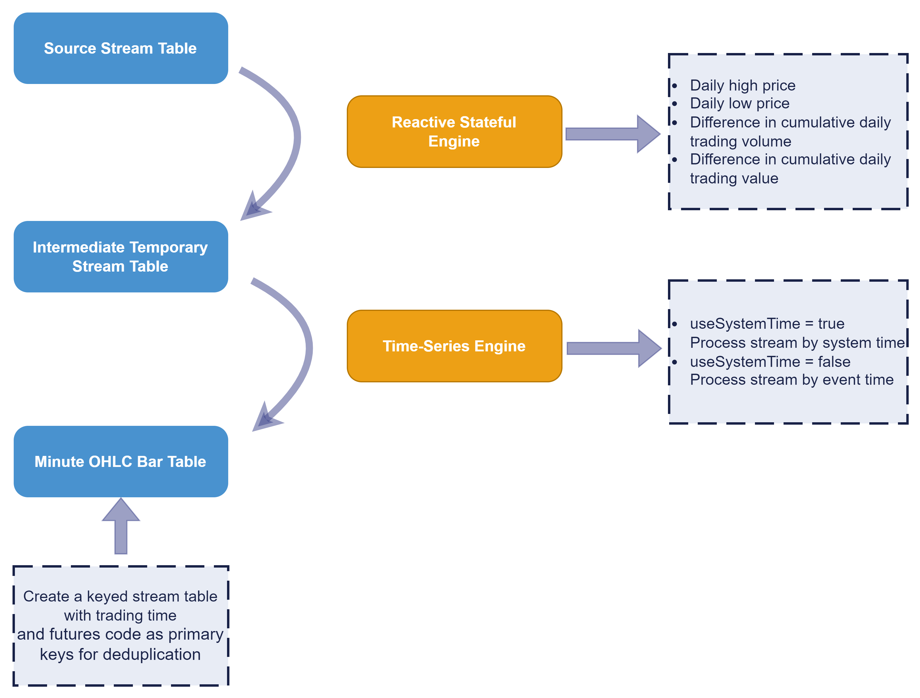
The flowchart for synthesizing OHLC bars based on real-time snapshot market data is as follows:
Next, we introduce the steps for building the futures snapshot data streaming computation framework. Detailed code is available in the streamFrame.dos in the appendix.
Step 1: Define the Raw Market Data Stream Table
First, create a source stream table with a schema consistent with the real-time data structure. Note: Before each run, you must clear the relevant stream tables and engines.
Explanation: When using the enableTableShareAndPersistence function, you must specify the configuration parameter persistenceDir in the configuration file (for standalone: dolphindb.cfg; for cluster: cluster.cfg). See Reference for details.
temp = streamTable(100:0, colNames , colTypes)
enableTableShareAndPersistence(table=temp, tableName=`quotationTable, cacheSize=1200000)
Step 2: Define the Intermediate Temporary Stream Table
First, define a temporary stream table to store the results computed by the reactive state engine. Then, use createReactiveStateEngine to create a reactive state engine that computes intermediate variables, such as the day's highest price, lowest price (using user-defined functions for high and low), the difference in cumulative daily trading volume, and the difference in cumulative daily trading value. Finally, subscribe to the raw market data stream so that data ingested into the raw stream table is published to the engine in real time, enabling the engine to process the raw data on the fly.
Step 3: Define the Minute-Bar Output Table and Compute Minute Data in Real Time Using a Time-Series Engine
First, create a keyed stream table using trading time and futures underlying code as primary keys. This target table ensures idempotent writes: writing records with the same key value multiple times produces the same result as the first write, thus preventing duplicate data. When adding new records to the table, the system automatically checks the primary key value of the new record:
-
If the primary key value of the new record duplicates an existing record in memory, the existing record is not updated.
-
When inserting multiple records in a single batch, if several records share the same primary key value (and that value does not match any existing record), only the first record is successfully inserted.
Next, use createTimeSeriesEngine to create a time-series stream engine, enabling real-time computation over a rolling time window. For example, to generate 1-minute OHLC bars, set the windowSize and step parameters to 60,000 milliseconds (i.e., 60 seconds).
After subscribing to the raw market data, the time-series engine inserts the computed results into the keyed stream table created earlier.
Step 4: Start Computation and Ingest Data into the Stream Table
// Assume the stream table is named: snapStream
objByName(`snapStream).append!(tb)
sleep(10000)
select top 100* from outputKlineTable
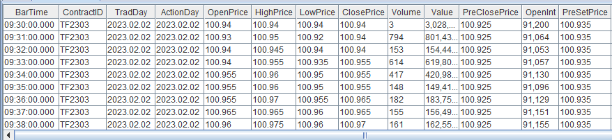
The following shows a sample of the 1-minute data in the stream table:
4. Futures Snapshot Data Minute-Level OHLC Bar Computation Module
In the previous sections, we detailed how to compute minute-level OHLC bars from historical futures snapshot data and how to synthesize continuous contract market data. Additionally, we introduced how to compute minute-level OHLC bars in real time within a streaming data scenario.
This section details the minute-level OHLC bar computation module FuturesOLHC. This module encapsulates the computation logic described above. By calling the module's functions, you can conveniently and efficiently perform historical computation of futures snapshot data, synthesize continuous contract market data, and perform real-time computation.
4.1 Module Structure and Features
The file structure of the FuturesOLHC DolphinDB module is as follows:
FuturesOLHC/
├── batchFrame.dos
├── createTable.dos
├── streamFrame.dos
├── tableSchema.dos
└── utils.dos
The function of each file is as follows:
| File Name | Description |
|---|---|
utils.dos |
Defines auxiliary functions used throughout the module |
tableSchema.dos |
Defines table schema functions for futures snapshot data and minute indicators |
createTable.dos |
Defines functions for creating corresponding partitioned tables |
batchFrame.dos |
Defines functions for calculating minute-level OHLC bars and continuous contract market data from historical futures snapshot data |
streamFrame.dos |
Defines functions for setting up the streaming computation framework for real-time futures snapshot minute-level OHLC bars |
4.2 Import Module
After downloading the DolphinDB module FuturesOLHC, you need to synchronize it to the server. When DolphinDB references the module, it searches the corresponding path for the required module file. For a detailed introduction to DolphinDB modules, refer to: Modules.
Synchronization Path
Place the module in the modules directory under the node's Home directory. You can obtain the node's Home directory via the getHomeDir function. Assuming the Home directory is /DolphinDB/server, you must place the module files under /DolphinDB/server/modules/.
How to Synchronize
-
Use file transfer tools (e.g., xftp) or DolphinDB clients such as GUI or the VS Code plugin to transfer the module to the specified path on the server.
-
Alternatively, use the scp command:
scp -r FuturesOLHC <user>@<server_ip>:/DolphinDB/server/modules/
4.3 How to Use the Module
The following sections detail the usage of the FuturesOLHC module. Complete sample code is available in the attachment: demo.dos
4.3.1 Create Partitioned Tables for Futures Snapshot Data and Minute-Level OHLC Bar Data
The following example demonstrates the creation of partitioned tables for snapshot data and minute-level data of commodity futures and treasury bond futures, based on the characteristics of their respective trading frequencies and market sizes:
// Import module file
use FuturesOLHC::createTable
// Database name for commodity futures snapshot data
comdtySnapDbname = "dfs://comdtySnapDb"
// Table name for commodity futures snapshot data
comdtySnapTbname = "comdtySnapTb"
// Database name for commodity futures minute-level data and continuous contract data
comdtyMinDbname = "dfs://comdtyMin"
// Table name for commodity futures minute-level data
comdtyMinTbname = "futurePrice1Min"
// Table name for commodity futures minute-level continuous contract data
comdtyZlTbname = "futurePrice1MinZl"

// Database name for treasury bond futures snapshot data
rtSnapDbname = "dfs://rtSnapDb"
// Table name for treasury bond futures snapshot data
rtSnapTbname = "rtSnapTb"
// Database name for treasury bond futures minute-level and continuous contract data
rtMinDbname = "dfs://rtMin"
// Table name for treasury bond futures minute-level data
rtMinTbname = "futurePrice1Min"
// Table name for treasury bond futures minute-level continuous contract market data
rtZlTbname = "futurePrice1MinZl"

// Create corresponding databases and tables based on specified parameters
createComdtyFuturesDfs(comdtySnapDbname, comdtySnapTbname)
createComdtyFuturesMinDfs(comdtyMinDbname, comdtyMinTbname)
createComdtyFuturesZlDfs(comdtyMinDbname, comdtyZlTbname)

createRtFuturesDfs(rtSnapDbname, rtSnapTbname)
createRtFuturesMinDfs(rtMinDbname, rtMinTbname)
createRtFuturesZlDfs(rtMinDbname, rtZlTbname)
Take the createComdtyFuturesDfs function, which creates partitioned tables for commodity futures minute bars, as an example. It requires two parameters:
| Parameter Name | Description |
|---|---|
| comdtyMinDbname | Database name |
| comdtyMinTbname | Table name |
For the specific code to create databases and tables, refer to the createTable.dos file in the FuturesOLHC module.
4.3.2 Build a Real-Time Futures Snapshot Data Streaming Engine
After creating the databases and tables, execute the following code to build the streaming engine and simulate the real-time computation process using the sample data provided in the attachment.
// Import module file
use FuturesOLHC::streamFrame
use FuturesOLHC::tableSchema
use FuturesOLHC::utils

// Raw commodity futures stream table name
rawComdtyStreamTbName = "comdtyStreamTb"
// Raw treasury bond futures stream table name
rawRtStreamTbName = "rtStreamTb"

try{
	// First, drop the persisted stream table
	unsubAndDropAll(rawComdtyStreamTbName)
    unsubAndDropAll(rawRtStreamTbName)
	// Then create the corresponding persisted stream table
	enableTableShareAndPersistence(table=createComdtyRawTable(), tableName=rawComdtyStreamTbName, cacheSize=10000)
    enableTableShareAndPersistence(table=createRTRawTable(), tableName=rawRtStreamTbName, cacheSize=10000)
}catch(ex){
	print(ex)
}

// Create the streaming engine for commodity futures snapshot data
nMin = 1 //Minute frequency (e.g., 1 indicates generating 1-minute-level OHLC bars)
dbname = comdtyMinDbname // Name of the target database for importing minute-level data
tbname = comdtyMinTbname // Name of the target table for importing minute-level data
FuturesOLHC::streamFrame::buildComdtyFrame(nMin, rawComdtyStreamTbName, dbname, tbname)


// Create the streaming engine for the treasury bond futures snapshot data
nMin = 1 //Minute frequency (e.g., 1 indicates generating 1-minute OHLC bars)
dbname = rtMinDbname // Name of the target database for importing minute-level data
tbname = rtMinTbname // Name of the target table for importing minute-level data
FuturesOLHC::streamFrame::buildRtFrame(nMin, rawRtStreamTbName, dbname, tbname)

// Path to commodity futures data files
comdtyPath = "/dolphindb/data/comdty_tickdata.csv"
// Get the stream table schema
sche = schema(objByName(rawComdtyStreamTbName,true)).colDefs
// Load sample data into an in-memory table
comdty_tickdata = loadText(comdtyPath,,sche)
// Replay sample data into the stream table
replay(comdty_tickdata, objByName(rawComdtyStreamTbName,true), `trd_ts, `trd_ts, -1, false)

// Path to treasury bond futures data files
rtPath = "/dolphindb/data/rt_tickdata.csv"
// Get the stream table schema
sche = schema(objByName(rawRtStreamTbName,true)).colDefs
// Load sample data into an in-memory table
rtTickdata = loadText(rtPath,,sche)
// Replay sample data into the stream table
replay(rtTickdata, objByName(rawRtStreamTbName,true), `trd_ts, `trd_ts, -1, false)
Take the buildComdtyFrame function, which creates a stream processing engine for commodity futures snapshot data, as an example. It takes four parameters:
| Parameter Name | Description |
|---|---|
| nMin | Minute granularity for calculation, e.g., 1 for 1 minute |
| rawComdtyStreamTbName | Name of the stream table for commodity futures snapshot data, into which upstream data is ingested |
| dbname | Database name for importing the computed minute-level OHLC bars |
| tbname | Table name for importing the computed minute-level OHLC bars |
For detailed steps on building the streaming engine, refer to Chapter 3. For the specific code, refer to the streamFrame.dos file in the FuturesOLHC module.
4.3.3 Compute Minute-Level OHLC Bars from Historical Futures Snapshot Data
This section uses sample data to demonstrate how to compute minute-level OHLC bars from historical futures snapshot data.
use FuturesOLHC::batchFrame

// Compute OHLC bars from historical commodity futures snapshot data
dataType = "cmdty"
dbname = comdtySnapDbname // Database name for storing historical raw data
tbname = comdtySnapTbname // Table name for storing historical raw data
// Load sample data into the database table
pt = loadTable(dbname, tbname)
pt.tableInsert(comdty_tickdata)

startDate = 2024.10.10 // Calculation start date
endDate = 2024.10.10 // Calculation end date
nMin = 1 //Minute frequency (e.g., 1 indicates generating 1-minute OHLC bars)
res  = getFuturesKMin(dataType, dbname, tbname, startDate, endDate, nMin)

// Compute OHLC bars from historical treasury bond futures snapshot data
dataType = "rt"
dbname = rtSnapDbname // Database name for storing historical raw data
tbname = rtSnapTbname // Table name for storing historical raw data
// Load sample data into the database table
pt = loadTable(dbname, tbname)
pt.tableInsert(rtTickdata)

startDate = 2024.10.08 // Calculation start date
endDate = 2024.10.08 // Calculation end date
nMin = 1 //Minute frequency (e.g., 1 indicates generating 1-minute OHLC bars)
res  = getFuturesKMin(dataType, dbname, tbname, startDate, endDate, nMin)
The function getFuturesKMin for computing minute-level OHLC bars from futures snapshot data takes six parameters:
| Parameter Name | Description |
|---|---|
| dataType |
Data category to compute
|
| dbname | Database name for storing historical futures snapshot data |
| tbname | Table name for storing historical futures snapshot data |
| startDate | Calculation start date |
| endDate | Calculation end date |
| nMin | Minute granularity for calculation, e.g., 1 for 1 minute |
For detailed calculation steps for generating minute-level OHLC bars from historical futures snapshot data, refer to Chapter 1; the specific code can be found in the FuturesOLHC module under the batchFrame.dos file.
4.3.4 Minute Continuous Contract Market Data Synthesis from Historical Futures Snapshot Data
This section uses sample data to demonstrate how to synthesize continuous contract market data from historical futures snapshot data.
// Commodity Futures Continuous Contract Market Data
minDbname = comdtyMinDbname
minTbname = comdtyMinTbname
zlDbname = comdtyMinDbname
zlTbname = comdtyZlTbname
startDate = 2024.10.10
endDate = 2024.10.10
nMin = 1
comdtyZL = comdtyZlFuturesKMin(minDbname, minTbname, zlDbname, zlTbname, startDate, endDate, nMin)

// Treasury Bond Futures Continuous Contract Market Data
minDbname = rtMinDbname
minTbname = rtMinTbname
zlDbname = rtMinDbname
zlTbname = rtZlTbname
startDate = 2024.10.08
endDate = 2024.10.08
nMin = 1
rtZL = rtZlFuturesKMin(minDbname, minTbname, zlDbname, zlTbname, startDate, endDate, nMin)
Here, taking the function comdtyZlFuturesKMin for synthesizing continuous contract market data from historical commodity futures snapshot data as an example, seven parameters are required:
| Parameter Name | Description |
|---|---|
| minDbname | Database name for storing minute bars of historical futures snapshot data |
| minTbname | Table name for storing minute bars of historical futures snapshot data |
| zlDbname | Database name for storing continuous contract market data from futures snapshot data |
| zlTbname | Table name for storing continuous contract market data from futures snapshot data |
| startDate | Calculation start date |
| endDate | Calculation end date |
| nMin | Minute granularity for calculation, e.g., 1 for 1 minute |
For detailed calculation steps for synthesizing continuous contract market data from historical futures snapshot data, refer to Chapter 2; the specific code can be found in the FuturesOLHC module under the batchFrame.dos file.
5. Summary
This tutorial details how to generate minute-level OHLC bars and continuous contract market data for futures using historical and real-time snapshot market data in DolphinDB. It also provides the FuturesOLHC module that implements the above functions, and then demonstrates in detail the steps for real-time calculation of minute-level OHLC bars, historical minute-level OHLC bar calculation, and continuous contract market data synthesis based on this module.
Note that the generation rules for OHLC bars and continuous contract market data described in this tutorial may differ from your actual use cases. You can refer to the module's source code in this tutorial and adjust it to your needs to quickly complete the project.
Appendix
-
Specific Trading Sessions for Different Futures Products:
Note:
This tutorial provides an overview of minute bar synthesis from Chinese futures snapshot data. For futures products with different trading sessions, you can modify the
getFuturesTradeTimefunction in theutils.doswithin the module to customize the trading sessions for the corresponding futures products.
| Futures Product | Futures Code | Trading Session |
|---|---|---|
| SSE 50 Index, CSI 300 Index, CSI 500 Index, CSI 1000 Index | IH,IF,IC,IM |
9:30—11:30 13:00—15:00 |
| No.1 Soybean, Common Wheat, Brent Crude Oil, Corn, Corn Starch, Styrene, Ethylene Glycol, Iron Ore, Coke, Coking Coal, Polyethylene, Soybean Meal, Palm Oil, Liquefied Petroleum Gas, Polypropylene, Paraxylene, Japonica Rice, Polyvinyl Chloride, Soybean Oil, Asphalt, Fuel Oil, Hot Rolled Coil, Rebar, Natural Rubber, Pulp, Thermal Coal, Cotton, Cotton Yarn, Glass, Methanol, Rapeseed Oil, Common Ferrosilicon, Rapeseed Meal, Ferrosilicon, White Sugar, Wire Rod, PTA | A,B,BR,C,CS,EB,EG,I,J,JM,L,M,P,PG,PP, PX,RR,V,Y,BU,FU,HC,RB,RU,SP,ZC,CF,CY,FG,MA,OI,PF, RM,SA,SR,SH,TA |
9:00—10:15 10:30—11:30 13:30—15:00 21:00—23:00 |
| Silver, Gold, Crude Oil | AG,AU,SC |
09:00—10:15 10:30—11:30 13:30—15:00 21:00—02:30 |
| Aluminum, Alumina, International Copper, Copper, Nickel, Lead, Tin, Stainless Steel, Zinc | AL,AO,BC,CU,NI,PB,SN,SS,ZN |
09:00—10:15 10:30—11:30 13:30—15:00 21:00—01:00 |
| Low Sulfur Fuel Oil, No. 20 Rubber | LU,NR |
09:00—10:15 10:30—11:30 13:30—15:00 21:00—23:00 |
| Apple, Red Date, Methanol, Japonica Rice, Late Indica Rice, Peanut, Common Wheat, Early Indica Rice, Rapeseed, Ferrosilicon, Manganese Silicon, Urea, Plywood, Fiberboard, Egg, Live Hog, Wire Rod, Strong Gluten Wheat, Polypropylene, Ferrosilicon | AP,CJ,EC,JR,LR,PK,PM,RI,RS,SF,SM,UR,BB, FB,JD,LH,WR,WH,LC,SI |
09:00—10:15 10:30—11:30 13:30—15:00 |
| 10-Year Treasury Bond Futures, 5-Year Treasury Bond Futures, 2-Year Treasury Bond Futures, 30-Year Treasury Bond Futures | T, TF, TS, TL |
09:30—11:30 13:00—15:15 |
-
Complete module for minute-level OHLC bar calculation from futures snapshot data
FuturesOLHC: FuturesOLHC.zip -
Example of minute-level OHLC bar calculation from futures snapshot data
demo.dos: demo.dos -
Sample data: data.zip