
Predict Realized Volatility in Real Time
Volatility measures the degree to which prices fluctuate over a given period. In real-time stock index futures trading, fast and accurate prediction of volatility over an upcoming period is critical for helping traders take timely and effective risk control and monitoring measures. Inspired by Kaggle's Optiver Realized Volatility Prediction Competition, this tutorial uses DolphinDB to build an end-to-end solution for storing high-frequency snapshot data from the Chinese stock market, preprocessing the data, building a model, and predicting volatility in real time.
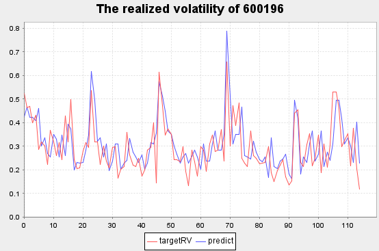
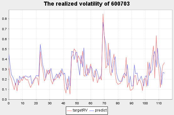
This tutorial uses 2020 level-2 snapshot data for the Shanghai Stock Exchange (SSE) 50 Index constituents to build high-frequency trading features at a 10-minute frequency, including bid-ask spread, depth imbalance, weighted average price, bid-ask pressure, and realized volatility. These features are used as model inputs, while the volatility over the next 10 minutes serves as the prediction target. A regression model is built with the adaBoostRegressor algorithm, which supports distributed computing in DolphinDB's built-in machine learning framework. Root Mean Square Percentage Error (RMSPE) is used as the evaluation metric. The final model achieves an RMSPE of 1.701 on the test set. The following figure shows selected volatility prediction results. The sample code in this tutorial requires DolphinDB Server v1.30.18+ or v2.00.6+.
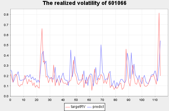
The trained model is persisted on the DolphinDB Server and used with DolphinDB's stream processing framework to predict the realized volatility of SSE 50 Index constituents over the next 10 minutes in real time.
1. Schema of Snapshot Data
This tutorial uses level-2 snapshot data from the SSE as its data source. Each snapshot is captured at an interval of 3 or 5 seconds. The data file has the following schema:
| Field | Description | Field | Description | Field | Description |
|---|---|---|---|---|---|
| SecurityID | Security symbol | LowPx | Low price | BidPrice[10] | Top 10 bid prices |
| DateTime | Date and time | LastPx | Last price | BidOrderQty[10] | Top 10 bid volumes |
| PreClosePx | Previous closing price | TotalVolumeTrade | Total trading volume | OfferPrice[10] | Top 10 ask prices |
| OpenPx | Opening price | TotalValueTrade | Total trading value | OfferOrderQty[10] | Top 10 ask volumes |
| HighPx | High price | InstrumentStatus | Trading status | ...... | ...... |
2. Data Preprocessing
The dataset imported into DolphinDB contains approximately 2.875 billion records and 174 columns. If you do not have snapshot data from the SSE, download the test data in the Appendix. For details on importing data into DolphinDB, see Data Import Method.
2.1 Data Sample Selection
This tutorial uses a subset of fields from the snapshot data, including stock symbol, snapshot time, as well as the top 10 bid prices, bid volumes, ask prices, and ask volumes.
The sample data consists of the SSE 50 Index constituents in 2020:
Stock symbol
601318,600519,600036,600276,601166,600030,600887,600016,601328,601288,
600000,600585,601398,600031,601668,600048,601888,600837,601601,601012,
603259,601688,600309,601988,601211,600009,600104,600690,601818,600703,
600028,601088,600050,601628,601857,601186,600547,601989,601336,600196,
603993,601138,601066,601236,601319,603160,600588,601816,601658,600745
2.2 Feature Engineering
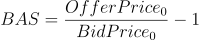
Bid-Ask Spread (BAS): Measures the spread between bid and ask prices.
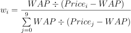
Weighted Average Price (WAP)

Depth Imbalance (DI)

Press: Bid-ask pressure



Feature data resampling (10-minute windows with aggregation of realized volatility)
Use group by SecurityID, interval(TradeTime, 10m, "none") for resampling.
Realized Volatility (RV): Realized volatility is defined as the standard deviation of logarithmic returns.

A stock's price always lies between the bid price and ask price. Therefore, this tutorial uses WAP instead of the stock price for calculations.
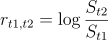
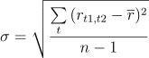
Because stock volatility is typically expressed on an annualized basis, the value must be annualized to obtain annualized realized volatility.

Because the data frequency is at the snapshot level, annualization requires multiplying the standard deviation by the square root of the number of snapshots in a full year.
2.3 Data Preprocessing Performance
2.3.1 OLAP Storage Engine
Data Preprocessing Code - OLAP
-
Total data volume in the DFS table: 2,874,861,174
-
Data volume for the SSE 50 Index constituents: 58,257,708
-
Data volume in the result table: 267,490
-
Logical CPU cores: 8
-
Elapsed time: 450 seconds
2.3.2 TSDB Storage Engine
Data Preprocessing Code - TSDB
The TSDB storage engine supports array vectors in DFS tables, whereas OLAP does not. Therefore, you can store the top 10 bid prices, bid volumes, ask prices, and ask volumes in four array vector columns, reducing the original 40 columns to 4 and significantly improving data compression, query performance, and computational performance.
-
Total data volume in the DFS table: 2,874,861,174
-
Data volume for the SSE 50 Index constituents: 58,257,708
-
Data volume in the result table: 267,490
-
Logical CPU cores: 8
-
Elapsed time: 40 seconds
Test results show that storing the top 10 bid prices, bid volumes, ask prices, and ask volumes as array vector columns in the TSDB storage engine makes computations 11 times faster than using the OLAP storage engine.
3. Model Building
Model Building and Training Code
Select adaBoostRegressor as the machine learning model.
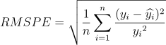
Evaluation metric: Root Mean Square Percentage Error (RMSPE)
Notes:
-
Except for
ols,pca,multinomialNB,kmeans, andknn, DolphinDB's machine learning functions take data sources generated by thesqlDSfunction as input. The data source specified bysqlDScan be an in-memory table or a DFS table. For machine learning functions that support distributed computing, ifsqlDSspecifies a DFS table as the data source, the system automatically distributes compute tasks among the servers that store the data and uses cluster resources to run them. -
The training result returned by
adaBoostRegressoris a dictionary that contains the following keys: numClasses, minImpurityDecrease, maxDepth, numBins, numTrees, maxFeatures, model, modelName, xColNames, learningRate, and algorithm. Here, model is a tuple that stores the trees generated during training, and modelName is "AdaBoost Classifier". -
The model generated by
adaBoostRegressorcan be passed to thepredictfunction for prediction.
3.1 Training and Test Sets
This tutorial does not use a validation set. The training and test sets are split as follows: train:test = 172029:73726.
login("admin", "123456")
dbName = "dfs://sz50VolatilityDataSet"
tbName = "sz50VolatilityDataSet"
dataset = select * from loadTable(dbName, tbName) where date(TradeTime) between 2020.01.01: 2020.12.31
def trainTestSplit(x, testRatio) {
 xSize = x.size()
 testSize =(xSize * (1-testRatio))$INT
 return x[0: testSize], x[testSize:xSize]
}
Train, Test = trainTestSplit(dataset, 0.3)
3.2 Training and Evaluation
def RMSPE(a,b)
{
 return sqrt(sum(((a-b)\a)*((a-b)\a))\a.size())
}
model = adaBoostRegressor(sqlDS(<select * from Train>), yColName=`targetRV, xColNames=`BAS`DI0`DI1`DI2`DI3`DI4`Press`RV, numTrees=30, maxDepth=16, loss=`square)
predicted = model.predict(Test)
Test[`predict]=predicted
print("RMSPE="+RMSPE(Test.targetRV,predicted))
Execution result:
RMSPE=1.701
Model training time: 25s
Hyperparameter tuning records
| RMSPE | trainTime (ms) | treeNum | maxDepth | features |
|---|---|---|---|---|
| 4.915 | 73240.025 | 60 | 20 | BAS,DI0-4,Press |
| 2.494 | 204696.819 | 60 | 32 | BAS,DI0-9,Press,RV |
| 2.778 | 323223.908 | 100 | 32 | BAS,DI0-9,Press,RV |
| 4.841 | 177327.831 | 60 | 32 | BAS,DI0-9,Press |
| 2.636 | 158605.04 | 60 | 32 | BAS,DI0-4,Press,RV |
| 1.974 | 51815.428 | 60 | 16 | BAS,DI0-4,Press,RV |
| 1.701 | 24782.163 | 30 | 16 | BAS,DI0-4,Press,RV |
| 1.878 | 13719.563 | 16 | 16 | BAS,DI0-4,Press,RV |
| 2.152 | 6854.556 | 8 | 16 | BAS,DI0-4,Press,RV |
Prediction performance of the regression model
| Number of Records | Inference Time (ms) |
|---|---|
| 1 | 0.614 |
| 10 | 2.271 |
| 100 | 11.446 |
| 1000 | 96.713 |
| 10000 | 959.438 |
The statistics above show that as the data volume increases, DolphinDB provides greater advantages for data processing and model prediction, enabling results to be generated quickly in stream processing scenarios.
3.3 Result Data Visualization
Randomly select one stock from the Test table and display the volatility prediction results from 2020.10.19 to 2020.10.23.
stock_id=(select distinct(SecurityID) from Test)[rand(50,1)[0]].distinct_SecurityID
plot((select targetRV,predict from Test where SecurityID=stock_id, date(TradeTime) between 2020.10.19: 2020.10.23), title="The realized volatility of"+stock_id,extras={multiYAxes: false})Notes:
-
The red line represents the actual values.
-
The blue line represents the predicted values.
Selected realized volatility prediction results for Fosun Pharma [600196] (a company listed on the SSE):
Selected realized volatility prediction results for San'an Optoelectronics [600703] (a company listed on the SSE):
4. Real-Time Volatility Prediction
4.1 Stream Processing Workflow
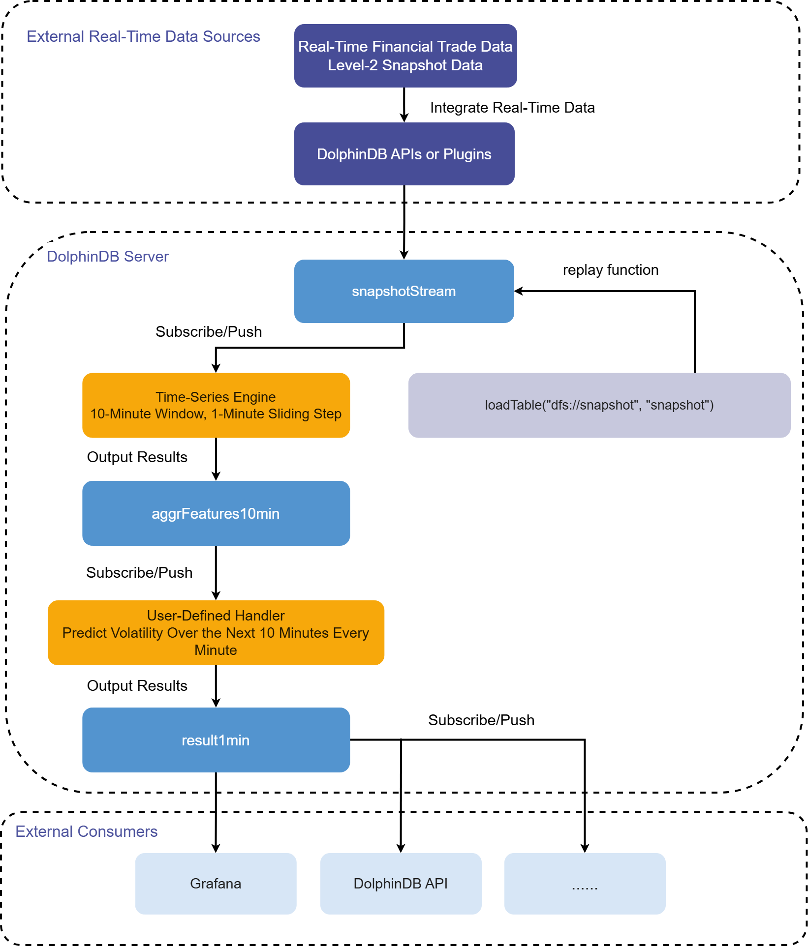
First subscription: Retrieves data from the snapshotStream table in real time and uses DolphinDB's time-series engine to perform sliding window aggregation with a 10-minute window and a 1-minute step. The core code is as follows:
-
Create a time-series engine
createTimeSeriesEngine(name="aggrFeatures10min", windowSize=600000, step=60000, metrics=metrics, dummyTable=snapshotStream, outputTable=aggrFeatures10min, timeColumn=`TradeTime, useWindowStartTime=true, keyColumn=`SecurityID) -
Subscribe to the snapshotStream stream table for real-time incremental data
subscribeTable(tableName="snapshotStream", actionName="aggrFeatures10min", offset=-1, handler=getStreamEngine("aggrFeatures10min"), msgAsTable=true, batchSize=2000, throttle=1, hash=0, reconnect=true)
Second subscription: Retrieves feature data from the processed aggrFeatures10min table in real time, uses the trained model to predict volatility, and writes the final results to the result1min table. The core code is as follows:
def predictRV(mutable result1min, model, msg){
 startTime = now()
 predicted = model.predict(msg)
 temp = select TradeTime, SecurityID, predicted as PredictRV, (now()-startTime) as CostTime from msg
 result1min.append!(temp)
}
subscribeTable(tableName="aggrFeatures10min", actionName="predictRV", offset=-1, handler=predictRV{result1min, model}, msgAsTable=true, hash=1, reconnect=true)
Third subscription: Pushes data from the result table result1min to external consumers in real time.
4.2 Demonstration
To help you quickly reproduce the real-time volatility prediction demo, this tutorial provides the model, data, and stream processing code. After downloading and extracting the zip file, store the model and data files on the DolphinDB Server, update the relevant path parameters in the code, and then quickly reproduce the stream processing workflow described above.
-
Trained models (select one based on your server version):
-
v1.30.18+:
realizedVolatilityModel_1.30.18.bin -
v2.00.6+:
realizedVolatilityModel_2.00.6.bin
-
-
Snapshot data (
testSnapshot.csv): 9,507 records for two stocks, 601319 and 600519, on October 19, 2020 -
Demo Code for Stream Processing
In the demo code, you must update the paths to the model file and data file.
/** modified location 1: modelSavePath, csvDataPath*/
modelSavePath = "/hdd/hdd9/machineLearning/realizedVolatilityModel_1.30.18.bin"
//modelSavePath = "/hdd/hdd9/machineLearning/realizedVolatilityModel_2.00.6.bin"
csvDataPath = "/hdd/hdd9/machineLearning/testSnapshot.csv"
4.3 Real-Time Monitoring with Grafana
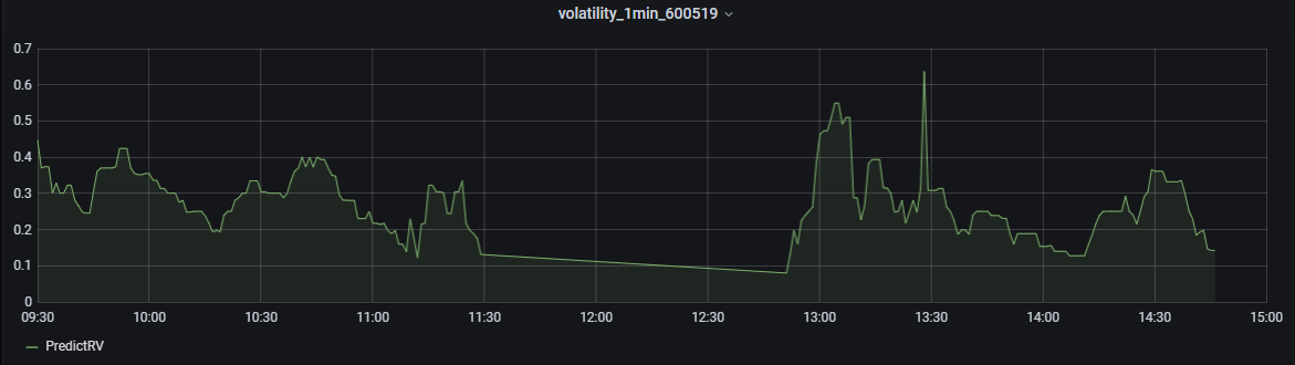
Query code in Grafana:
select gmtime(TradeTime), PredictRV from result1min where SecurityID=`600519Note: Grafana uses UTC as the default time zone, which may differ from the data timestamp in the DolphinDB Server depending on the server’s local time zone. Therefore, the query in Grafana must use the gmtime function for time zone conversion.
4.4 Real-Time Prediction Latency
In a real-world scenario that predicts volatility for SSE 50 Index constituents in real time, snapshot data is generated at a rate of approximately 1,000 records per minute. Run the following statement on the result table result1min to query prediction latency:
select avg(CostTime) as avgCostTime, min(CostTime) as minCostTime, max(CostTime) as maxCostTime from result1minQuery result:
| avgCostTime | minCostTime | maxCostTime |
|---|---|---|
| 13 ms | 7 ms | 18 ms |
5. Summary
This tutorial uses DolphinDB's powerful data processing capabilities, easy-to-use machine learning framework, and stream processing framework to implement real-time stock volatility prediction. Compared with traditional data processing and model-building approaches such as Python-based solutions, DolphinDB tightly integrates its storage engines and compute engines, making it easy to perform distributed parallel computing during data preprocessing and model training. This reduces memory usage while improving computational efficiency.
Together with DolphinDB's stream processing framework, this tutorial provides a complete and efficient solution for similar production requirements, including data processing, model training, and real-time prediction. In this tutorial, the system subscribes to level-2 snapshot data for the SSE 50 Index constituents. As real-time data is generated, it can predict the volatility of each stock over the next 10 minutes within 13 ms, guiding the development of trading strategies.
6. Appendix
Note: The sample code in this tutorial must run on DolphinDB Server v1.30.18+ or v2.00.6+.
6.1 Scripts
6.2 Models
6.3 Data
6.4 Production Environment
-
CPU: Intel(R) Xeon(R) Silver 4216 CPU@2.10GHz
-
Total logical CPU cores: 8
-
Memory: 64 GB
-
OS: 64-bit CentOS Linux 7 (Core)
-
Disk: SSD, with a maximum read/write speed of 520 MB/s
-
Server version: v1.30.18+, v2.00.6+
-
Server deployment mode: standalone
-
Configuration file for v1.30.18+: dolphindb.cfg (volumes and persistenceDir must be updated based on the disk paths in your environment)
-
Configuration file for v2.00.6+: dolphindb.cfg (volumes, persistenceDir, and TSDBRedoLogDir must be updated based on the disk paths in your environment)
-
Standalone deployment tutorial: Standalone Deployment and Upgrade