Technical Principles of the Orca Real-Time Computing Platform

DolphinDB already has comprehensive stream computing capabilities: stream tables receive data, the publish-subscribe mechanism transfers data, and engines such as the time-series engine, reactive state engine, and join engine perform computation, while persistence and high availability (HA) mechanisms ensure reliability. When the business scenario is simple, developers can complete the task by directly creating these objects. Problems arise as the business becomes more complex.

Take real-time market data processing as an example. After tick-by-tick trades enter the system, it may need to generate 1-minute, 5-minute, and intraday multi-period OHLC bars at the same time. The resulting OHLC bars may then feed into moving-window indicators, rule checks, risk monitoring, persistence, and downstream subscriptions. From a business perspective, this is a clear data processing pipeline. When implemented in scripts, however, it often turns into multiple input tables, intermediate tables, output tables, engines, and subscription relationships, plus node deployment and restart recovery logic.

What is even harder to maintain are the relationships between these objects. Before the system can truly be deployed to production, the following questions need careful consideration: which tables and engines belong to the same business pipeline, which objects must be created first, whether stopping a task means stopping the input first or deleting intermediate objects first, and where to restore subscription offsets (that is, the record from which consumption resumes) and engine states after a node failure.

If all these relationships are embedded in user scripts, the larger the system, the more likely it is that problems occur: the computation logic itself is not wrong, but the deployment order, recovery order, or object cleanup goes wrong. At best, these problems are merely hard to troubleshoot; at worst, they cause incidents such as duplicate consumption, some pipeline branches still writing data, and downstream consumers seeing inconsistent results.

This is exactly the kind of problem Orca solves. Users only need to submit a stream graph—a complete description of a real-time computation task—specifying where data comes from, what computations it goes through, and where it is finally written. Based on this graph, Orca generates the stream tables, engines, subscriptions, tasks, node deployment plan, and recovery plan needed for actual execution. This way, developers only need to maintain the business data flow, while Orca handles the error-prone details of distributed execution.

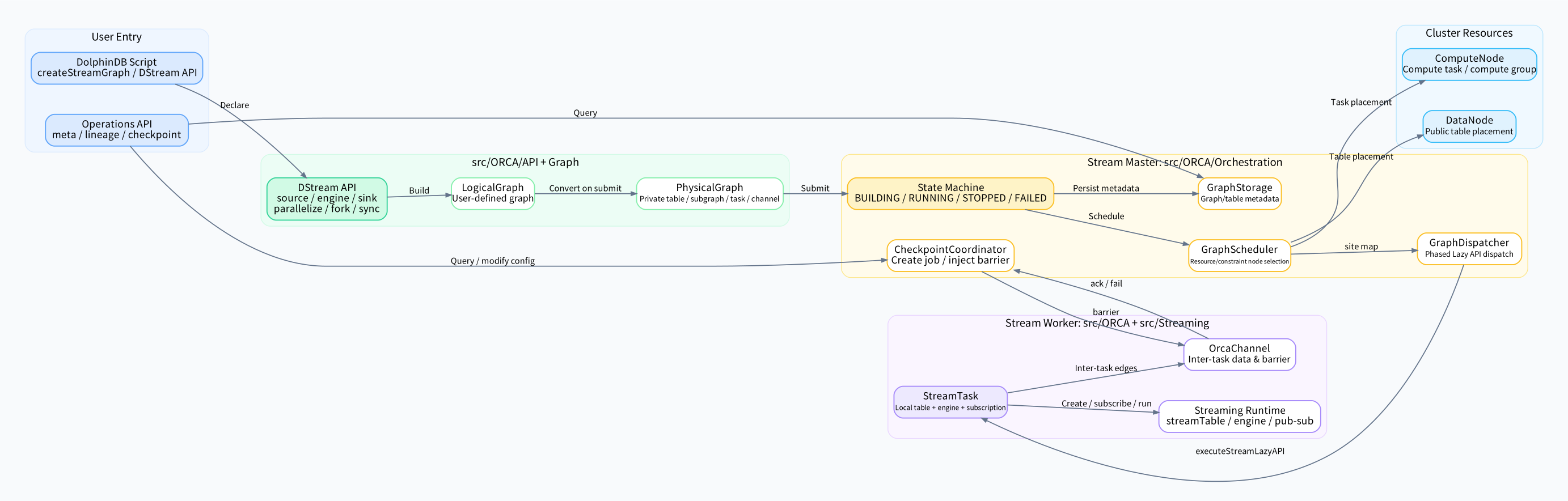
A stream graph is a complete description of a real-time computation task in Orca. It manages input tables, computation engines, intermediate results, output tables, and the data flow relationships among them in a single graph.

When writing a stream graph, developers mainly use the following types of interfaces:

• Input: source (and variants such as keyedSource and haSource) corresponds to a public stream table that can be written to externally.

• Computation: engine interfaces such as timeSeriesEngine and reactiveStateEngine. Internally, these are still DolphinDB's existing streaming engines.

• Visible intermediate result: buffer materializes the intermediate result of a step into a public stream table. By default, intermediate results between engines are carried by Orca internal objects and are not visible externally. Once you explicitly mark it with buffer, the result of that step becomes a public stream table that can be queried and subscribed to externally. Further computation can continue after it.

• Output: sink connects the current step to a public stream table, a DFS table, or a function.

• Branch/parallelize: fork duplicates the same data into multiple paths; parallelize splits data by specified columns for parallel computation, and then sync merges the results.

When writing a stream graph, developers care about the business pipeline: trade data enters the system, is aggregated in parallel by stock symbol, is turned into OHLC bars, then goes through moving-window indicators, and is finally written to an output table. After receiving this graph, Orca can validate the structure before submission, split tasks at submission time, maintain state during runtime, and recover from the metadata after a failure.

Abstracting the stream processing pipeline into a stream graph allows Orca to do much more than ordinary script encapsulation. At submission time, it checks whether table schemas (column names and types) are consistent and whether the use of source and sink is valid. At scheduling time, it can see the parallelism and node constraints of the whole graph. When stopping or destroying a graph, it can close subscriptions, tables, and engines in dependency order. When a failure occurs, it can recover the original runtime structure from metadata and checkpoint information (a checkpoint is the unified recovery point of the entire graph). Script encapsulation merely hides the actions of creating tables, engines, and subscriptions. A stream graph, in contrast, saves the business relationships behind those actions, enabling subsequent scheduling, recovery, and troubleshooting by the system.

From an implementation perspective, Orca is built on top of the streaming subsystem. Data processing is still done by DolphinDB's existing streaming engines. What Orca adds is management capability around stream graphs, including graph construction, scheduling, distribution, permissions, recovery, and checkpoints. This lets Orca reuse the mature stream processing capabilities while putting distributed orchestration in a separate layer.

At runtime, Orca can be viewed as consisting of two parts. The Stream Master is responsible for storing metadata, generating the physical graph, scheduling stream tasks (the smallest unit actually deployed to a node for execution; see Section 4.3), dispatching construction actions to nodes, and coordinating checkpoints. It does not participate in data computation. Worker nodes are responsible for actually creating stream tables, engines, subscriptions, and the data channels (Orca Channels) used to transfer data between tasks. Orca Channels are internal objects automatically inserted by the system and do not appear in user scripts. When two tasks are not in the same contiguous computation chain and data must flow from one task to another, the system inserts a channel between them. The channel carries both ordinary data and checkpoint progress markers. Data mainly flows between worker nodes. The Stream Master does not participate in data computation; it is responsible for overall scheduling and permission control.

When developers write a stream graph, they describe business logic. The example below shows a pipeline that takes trade data as input, generates OHLC bars, calculates several moving-window indicators, and finally writes to an output table. The function used at each step is marked in the comments.

if (!existsCatalog("Orca")) {
    createCatalog("Orca")   // catalog: provide a namespace for the stream graph, tables, and engines
}
go
use catalog orca

// createStreamGraph: create a stream graph named graph1
g = createStreamGraph(`graph1)

// source: define the input table Trade; if the table already exists, validate its schema
// timeSeriesEngine: aggregate OHLC bars in 1-minute windows
// reactiveStateEngine: calculate rolling indicators on OHLC bars
// sink: write the result to the output table named output
g.source("Trade", `symbol`datetime`price`volume, [SYMBOL, TIMESTAMP, DOUBLE, INT])
 .timeSeriesEngine(
 60*1000, 60*1000,
 <[first(price), max(price), min(price), last(price), sum(volume)]>,
 "datetime", false, "symbol")
 .reactiveStateEngine(
 <[datetime, first_price, max_price, min_price, last_price, sum_volume,
 mmax(max_price, 5), mavg(sum_volume, 5)]>,
 `symbol)
 .sink("output")
// submit: pass the logical graph to Orca, which deploys and starts it in the cluster
g.submit()

This script does not specify whether private stream tables need to be created in the middle, how to subscribe across nodes, how parallel tasks are numbered, or when the source subscription should start. For developers, these details should not be mixed into business logic; in production, however, they must be handled explicitly.

After submit() is called, Orca converts the user-written logical graph into a physical graph. The logical graph answers what computation should be applied to the data; the physical graph answers how this data pipeline runs in the cluster. The conversion sequence is roughly as follows: first, check whether the graph is valid (for example, whether it contains cycles and whether each engine has a downstream output); then add necessary intermediate tables and remove redundant ones; split the graph into several subgraphs (a subgraph is a section cut out of the whole stream graph; see Section 4.3); split it into stream tasks according to the degree of parallelism; and finally insert Orca Channels wherever data must be transferred across subgraphs.

This separation is similar to the way SQL is used in databases. When writing SQL, users only describe what to query, and the optimizer generates an execution plan. In Orca, the chained data stream (DStream) written by the user describes the business data flow, and the physical graph generates a deployable, schedulable, recoverable stream processing execution plan.

With this separation, the business expression can remain stable while the execution approach can continue to evolve. Later, if parallelism, node distribution, checkpoint policy, or scheduling policy changes, these details do not need to be exposed back to business scripts.

Before a graph can actually run, Orca must first translate business logic into the runtime objects that will run in the cluster. This step must answer the following questions:

• Which runtime objects does each source, engine, or sink ultimately map to?

• Which objects can run together in the same node, and which must be split across different nodes or tasks?

• Which locations need intermediate stream tables to relay data?

• Which cross-node data flows need Orca Channel?

• Which objects should be created first, and which should be created later?

If these issues were left to users to handle by writing scripts manually, the work would be tedious and highly error-prone. Orca performs these transformations in a unified manner during submission.

use catalog orca

g = createStreamGraph("engine_fork_demo")

// The same time series engine feeds two downstream branches.
eng = g.source(
 "Trade",
 `symbol`datetime`price`volume,
 [SYMBOL, TIMESTAMP, DOUBLE, INT]
).timeSeriesEngine(
 60*1000, 60*1000,
 <[first(price), max(price), min(price), last(price), sum(volume)]>,
 "datetime", false, "symbol")

// fork(2): duplicates the current engine's output into two branches; count must be greater than 1.
branches = eng.fork(2)

branches[0]
    .sink("output_kline")          // One branch writes directly to OHLC bars.

branches[1]
    .reactiveStateEngine(          // The other branch continues computing rolling indicators.
 <[datetime, first_price, max_price, min_price, last_price, sum_volume,
 mmax(max_price, 5), mavg(sum_volume, 5)]>,
 `symbol)
 .sink("output_indicator")

g.submit()

Scheduling answers the question: after a graph is split into multiple execution tasks, on which node should each task be placed? This decision cannot be made by looking only at which nodes are idle; it must also consider what the task itself requires.

Some requirements come from table placement. Public stream tables are normally placed on data nodes because they must be read and written externally and will also persist as metadata over the long term. If a task depends on an existing public stream table, the scheduler tries to place the task close to that table to reduce unnecessary cross-node access.

Some requirements come from compute resources. Compute tasks can be placed on data nodes or compute nodes. If the user specifies a compute group, the isolation constraints of that compute group must be followed, and the task cannot be arbitrarily placed into another compute resource group.

Shared variables in user-defined functions (UDFs) are another type of constraint that requires special handling. UDFs can read and write shared state such as shared tables, shared dicts, and shared keyed tables. If tasks accessing the same shared state are distributed across multiple nodes, it creates problems of cross-node consistency, locking, replication, and recovery. Currently, during the scheduling phase, Orca places these tasks in the same constraint group and tries to put them on the same node. The primary purpose is clear execution semantics, not merely performance optimization.

After these constraints are satisfied, the scheduler examines the node's current load, remaining memory, disk space on data nodes, network I/O, and the weights of preferred nodes. The current implementation uses heuristic scoring and does not aim for a globally optimal solution. For stream graphs submitted online, scheduling needs to be fast enough, stable enough, and easy to explain. Strictly optimal scheduling would require modeling future traffic, state sizes, network costs, and failure probabilities, which is expensive and may not yield stable practical benefits.

The scheduling implementation also deducts node scores based on task complexity. Once a node has been assigned a task, its subsequent score is lowered to prevent all tasks from being placed on the node with the highest initial score.

After scheduling, the system has only determined which node each task should run on; the stream graph is not actually running yet. The next step is to create the stream tables, engines, and subscription relationships corresponding to these tasks on the target nodes.

Orca does not start all objects at once. Instead, it performs the startup in several steps:

1. Creates the local stream tables and engines, preparing the compute chain inside each task.

2. Creates non-source subscriptions, so that intermediate and downstream links are connected first.

3. Creates the source subscriptions so that input data enters the entire graph.

The purpose of this order is mainly to avoid a partially started state. In a real-time computation pipeline, once the entry is opened, data flows in continuously. If a source subscription starts before downstream tables or engines are ready, the system may end up with some data having already entered while some links are not yet connected. Later, when troubleshooting, users will see not a clean startup failure but an incomplete pipeline state.

Order must also be considered when destroying objects. The system first stops subscriptions and then deletes tables and engines, preventing a situation where upstream is still pushing data after an object has already been deleted.

These creation and destruction actions are expressed through the deferred execution interface (Lazy API). The stream master does not need to directly manipulate C++ objects on remote nodes. It only generates a set of descriptions of what actions the node should perform and passes them to the corresponding worker node for execution. After the worker node completes execution, it returns the task status and error reason to the stream master. This way, whether for submission, recovery, or destruction, the system can reuse the same execution mechanism. On failure, it can also clearly identify which stage and which task the problem occurred in.

From submission to destruction, a stream graph goes through several stages: creating metadata, deploying tasks, entering the running state, stopping, restarting, resubmitting, and finally destroying. Each step affects metadata and also affects the stream tables, engines, and subscription relationships distributed across multiple nodes, so this cannot be treated as an ordinary function call.

Taking submission as an example, the system must save the serialized graph data (graph blob), update the graph metadata, create or update public stream table metadata, record which node each task is assigned to, and record whether each task is currently running successfully or has failed. If checkpointing is enabled, the checkpoint configuration must also be associated with this graph. If any step fails, the system must know which stage the failure occurred in.

If these states are not recorded clearly, partially completed states can easily occur: for example, tables have been created but the metadata has not been updated; some tasks are running but the graph still shows a building state; or, when the graph is being destroyed, subscriptions are not stopped cleanly, and data continues to be written to objects that have already been deleted.

The stream master chains these steps together and records the current phase of the graph and its tasks. This way, when users call functions such as startStreamGraph, stopStreamGraph, and resubmitStreamGraph, they do not need to determine which subscriptions should be stopped first, which tables and engines can be kept, or which step to restart from after a failure. The system will perform the corresponding start, stop, or resubmission based on the current state.

During failure recovery, the system needs to ensure that all tasks return to the same processing point. For example, the upstream may have processed up to the 10,000th record while the downstream has only processed up to the 9,800th, with a batch of unprocessed data still in the intermediate channel. If each node saves its own state independently, recovery can result in missing data or reprocessing.

Checkpointing solves exactly this problem: it establishes a unified recovery point for the entire stream graph. Orca uses a barrier to mark this point. The checkpointing component injects barriers from the source side. Barriers travel downstream on the same path as ordinary data.

When a task receives a barrier, it means that, on that input, all data preceding the barrier has already been processed. The task then saves its own state and returns the result of the save. The checkpoint is considered successful only after all related tasks have completed saving state and returned their results.

The situation becomes more complicated if a task has multiple upstream inputs. It cannot assume that it can save state just because one input has reached a barrier, because another input may still be at an earlier point. In this case, Orca Channel temporarily holds the barrier that arrived first, and only after the other inputs have also received a barrier from the same checkpoint does it allow the task to save its state and continue processing. This way, when recovery occurs, all inputs correspond to the same processing point.

During recovery, Orca can rebuild the graph state and processing progress from the most recent successful checkpoint. Because the system records a unified recovery point, users do not need to check the progress of each engine, subscription, or intermediate channel one by one, nor do they need to manually assemble scattered state from multiple nodes.

Real-time computation tasks usually run for a long time. After submission succeeds, users also need ongoing visibility into its status: whether the graph is still running, which computations produce the output tables, and which tasks are affected when a node fails. When users need to stop or restart a stream graph, there should also be a single control point rather than requiring them to handle each table, engine, and subscription individually.

Without unified metadata, troubleshooting means going back to inspect scripts, review subscription settings, and check the status and logs of individual nodes. Orca solves this by registering graphs, tables, and engines in a catalog, making them queryable and manageable objects. As a result, users see not only variables created in a session, but a set of real-time computing resources with names, metadata, and lifecycles.

With this metadata, troubleshooting can start from the stream graph. You can inspect the graph to see whether it is running, failed, or stopped; inspect a table to see which node hosts a given Orca stream table and which graphs reference it; inspect checkpoints to see which task the recovery process is stuck on; and inspect data lineage to see which graph produced an output table and what computations it went through.

Permissions can also be controlled per object. Compute groups mainly restrict the computing resources a task can use; Orca graph, table, and engine permissions control who can create or stop graphs, read or write Orca stream tables, and manage engines. This makes it possible to restrict both the resources on which tasks can run and the real-time computing objects that users can operate on.

The multi-period OHLC bar example below ties together the preceding process. The business goal is to ingest tick-by-tick trades from Trade, generate 1-minute and 5-minute OHLC bars, compute moving indicators, and write the results to two Orca output tables.

if (!existsCatalog("orca")) {
 createCatalog("orca")
}
go
use catalog orca

g = createStreamGraph(`kline_graph)

sourceStreams = g.source(
 "Trade",
 `symbol`datetime`price`volume,
 [SYMBOL, TIMESTAMP, DOUBLE, INT]
).fork(2)

stream_1min = sourceStreams[0]
 .parallelize("symbol", 4)
 .timeSeriesEngine(
 60*1000, 60*1000,
 <[first(price), max(price), min(price), last(price), sum(volume)]>,
 "datetime", false, "symbol")
 .reactiveStateEngine(
 <[datetime, first_price, max_price, min_price, last_price, sum_volume,
 mmax(max_price, 5), mavg(sum_volume, 5)]>,
 `symbol)
 .sync()
 .sink("output_1min")

stream_5min = sourceStreams[1]
 .parallelize("symbol", 4)
 .timeSeriesEngine(
 5*60*1000, 5*60*1000,
 <[first(price), max(price), min(price), last(price), sum(volume)]>,
 "datetime", false, "symbol")
 .reactiveStateEngine(
 <[datetime, first_price, max_price, min_price, last_price, sum_volume,
 mmax(max_price, 5), mavg(sum_volume, 5)]>,
 `symbol)
 .sync()
 .sink("output_5min")

g.submit()

Before submission, the script only describes the business pipeline: Trade is the input, data is split into two branches that compute 1-minute and 5-minute OHLC bars, and the results are written to two output tables. At this point, intermediate tables, node selection, subscription order, and failure recovery are not yet involved.

After submit() is called, Orca begins converting this business pipeline into a structure that can run on the cluster. The system first checks the graph and table structures, then generates the physical graph. Private stream tables are inserted where intermediate buffering is needed, Orca Channels are inserted where data must cross task boundaries, and portions parallelized by symbol are split into multiple schedulable stream tasks.

The system then saves metadata for the graphs and tables, so the pipeline can be queried, stopped, restarted, and recovered. The scheduler then selects a node for each task based on table location, node resources, compute groups, shared state, and other conditions.

During deployment, Orca creates the stream tables, engines, and subscriptions on the target nodes in order: it prepares the intermediate and downstream pipeline components first, and opens the source subscription last. This way, when data begins to be written to Trade, the downstream 1-minute and 5-minute branches are already ready to receive it and continue computing, and the results eventually flow into output_1min and output_5min.

If checkpointing is enabled, barriers propagate downstream together with data from source; cross-task pipelines are handled by Orca Channel, ensuring that all tasks save the same processing progress. During later recovery, Orca can restore the state inside the graph from the last successful checkpoint.

This example captures the division of responsibilities in Orca: developers write business logic, and Orca is responsible for turning it into the tables, engines, subscriptions, tasks, channels, metadata, and recovery logic needed for actual execution.