Calculate Minute-Level Capital Flow in Real Time
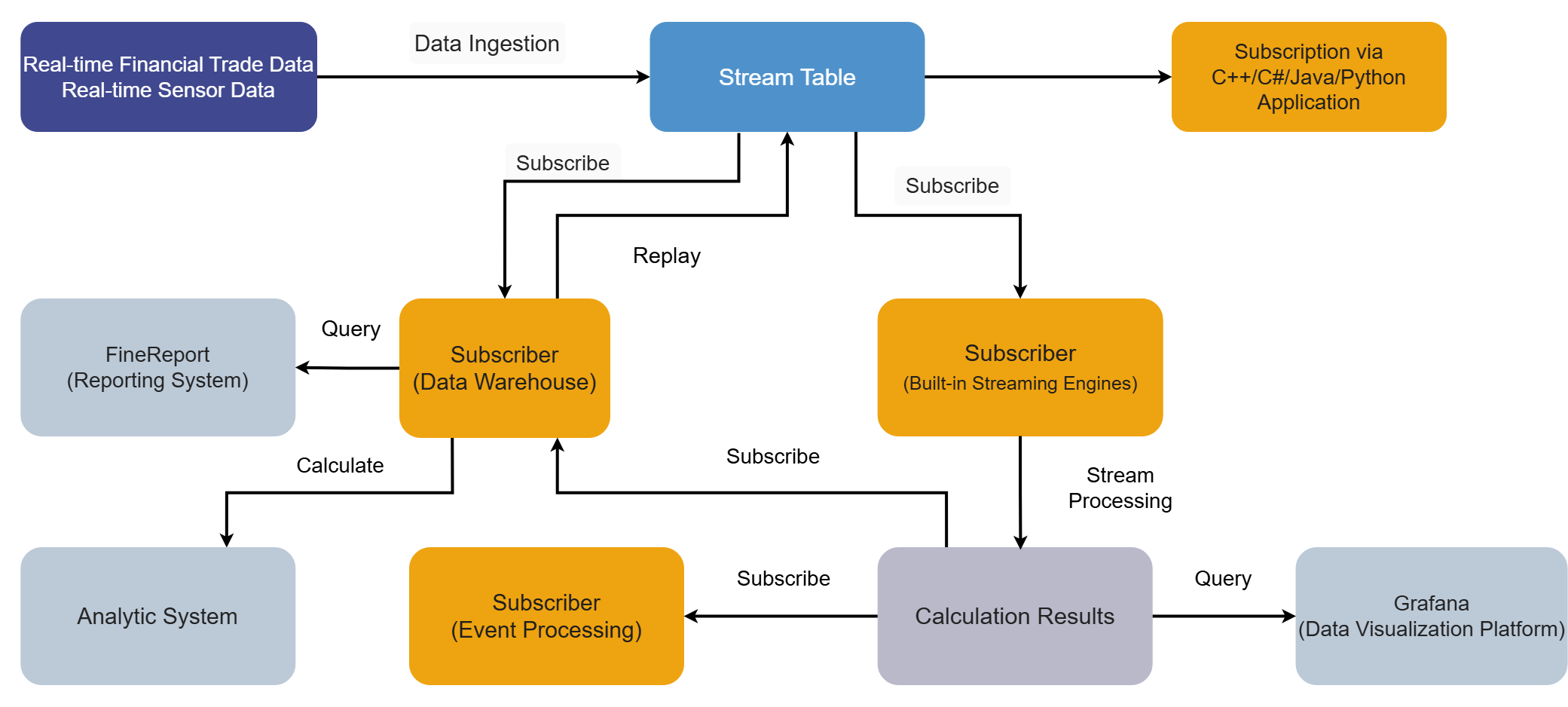
DolphinDB's built-in stream processing framework combines high performance with ease of use. It supports publishing, subscribing to, and preprocessing streaming data, performing real-time in-memory calculations, and calculating complex metrics over rolling, sliding, and cumulative windows. This tutorial describes how to use this framework to calculate minute-level capital flow in real time.
1. Scenario Overview
Using simulated tick-by-tick trades from the Shanghai Stock Exchange (SSE) on a trading day in 2020 as the data source, this tutorial demonstrates how to calculate minute-level capital flow in real time with DolphinDB's stream processing framework. This example calculates the trading value of large and small orders (buy or sell) over a 1-minute rolling window, classifying orders by trading volume with a threshold of 50,000 shares.
1.1 Data Source
The schema of the DolphinDB table used to store tick-by-tick trades from SSE is as follows:
| Column Name | Data Type | Description |
|---|---|---|
| SecurityID | SYMBOL | Stock code |
| Market | SYMBOL | Exchange |
| TradeTime | TIMESTAMP | Trade time |
| TradePrice | DOUBLE | Trade price |
| TradeQty | INT | Trading volume |
| TradeAmount | DOUBLE | Trading value |
| BuyNum | INT | Buy order number |
| SellNum | INT | Sell order number |
1.2 Metrics
This tutorial calculates the following metrics:
| Metric Name | Description |
|---|---|
| BuySmallAmount | Trading value of buy-side small orders over the past 1 minute, where trading volume is less than or equal to 50,000 shares. |
| BuyBigAmount | Trading value of buy-side large orders over the past 1 minute, where trading volume is greater than 50,000 shares. |
| SellSmallAmount | Trading value of sell-side small orders over the past 1 minute, where trading volume is less than or equal to 50,000 shares. |
| SellBigAmount | Trading value of sell-side large orders over the past 1 minute, where trading volume is greater than 50,000 shares. |
Rules for classifying large and small orders in capital flow analysis vary across stock market software, but they are generally based on the quantity of shares traded or the trading value. For example, common stock market software in China uses the following rules:
-
Eastmoney
-
Extra-large order: >500,000 shares or CNY 1,000,000
-
Large order: 100,000-500,000 shares or CNY 200,000-1,000,000
-
Medium order: 20,000-100,000 shares or CNY 40,000-200,000
-
Small order: <20,000 shares or CNY 40,000
-
-
Sina Finance
-
Extra-large order: >CNY 1,000,000
-
Large order: CNY 200,000-1,000,000
-
Small order: CNY 50,000-200,000
-
Very small order: <CNY 50,000
-
In this tutorial, orders are classified solely by trading volume into two categories: large and small. The threshold is set arbitrarily for demonstration purposes, so you must adjust it to suit your actual use case.
1.3 Real-Time Calculation Solution
This tutorial calculates capital flow in real time by using a user-defined aggregate function. The processing workflow in DolphinDB is shown below:
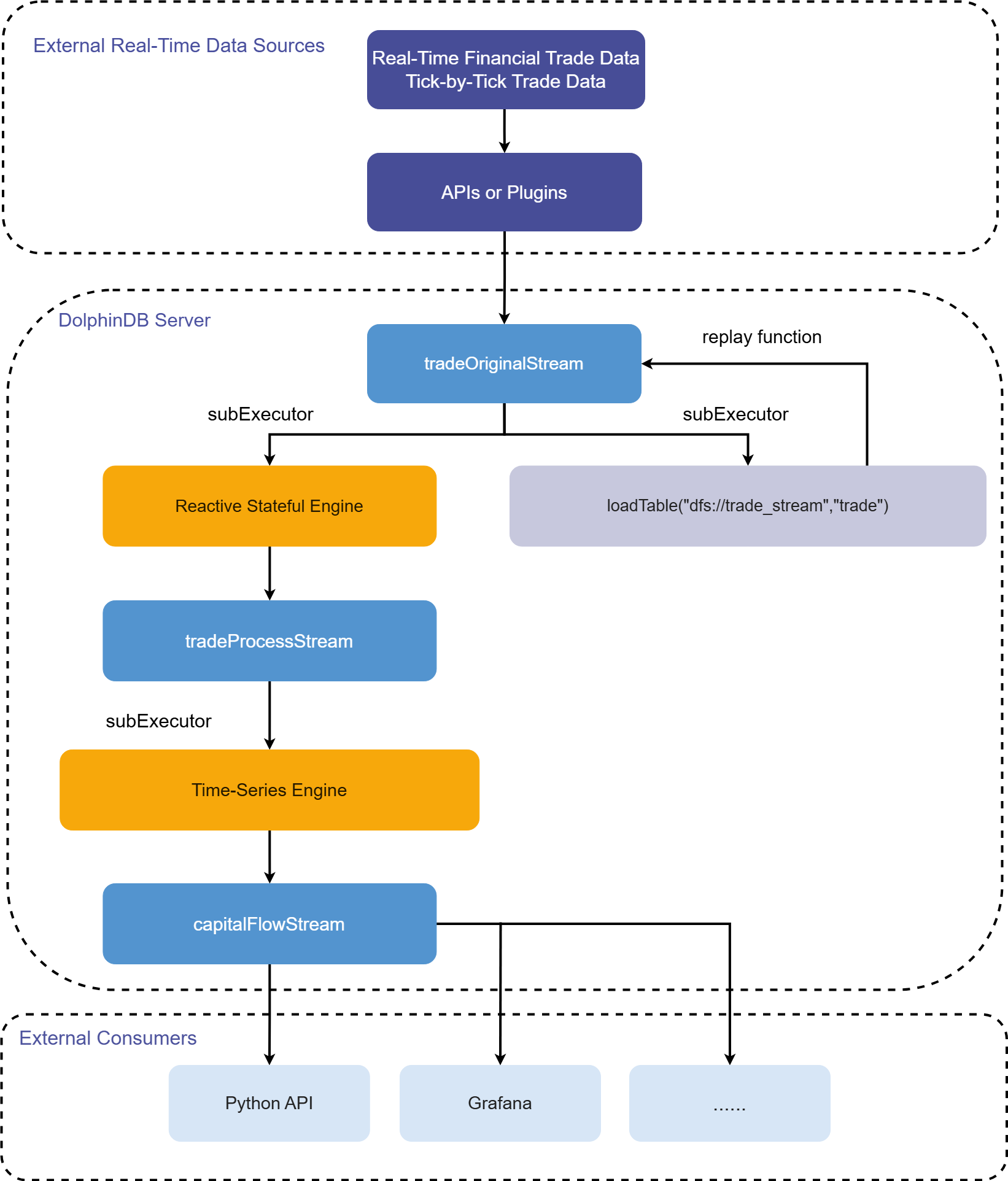
Workflow description:
-
tradeOriginalStream, tradeProcessStream, and capitalFlowStream are all shared asynchronously persisted stream tables.
-
tradeOriginalStream: Receives and publishes real-time streaming data for tick-by-tick stock trades.
-
tradeProcessStream: Receives and publishes intermediate data processed by the reactive stateful engine.
-
capitalFlowStream: Receives and publishes capital flow metrics for a 1-minute rolling window processed by the time-series engine.
-
Share in-memory tables so they are accessible to all other sessions on the current node. When real-time streaming data is written to DolphinDB stream tables through the API, the session connected to the DolphinDB server may differ from the session that defined the tables, so the tables must be shared.
-
Persisting a stream table serves two main purposes. First, it limits the table's maximum memory usage. By setting the cacheSize parameter in the
enableTableShareAndPersistencefunction, you can control the maximum number of records retained in memory and therefore the table's maximum memory usage. Second, in the event of an unexpected node shutdown, you can recover data that was written to the stream table but not yet consumed from the persisted data files, ensuring the streaming data is consumed at least once. -
Stream tables use asynchronous persistence, which effectively improves write throughput. Only stream tables can be subscribed to and consumed, so tradeOriginalStream, tradeProcessStream, and capitalFlowStream must all be defined as stream tables.
-
-
subExecutor refers to a stream processing thread.
-
Set the subExecutors parameter in the configuration file to specify the maximum number of stream processing threads available on the node.
-
Set the hash parameter in the
subscribeTablefunction to specify which stream processing thread consumes the topic. For example, if subExecutors is set to n, you can set hash to any value from 0 to n-1, corresponding to stream processing threads 1 to n.
-
-
The reactive stateful engine and time-series engine are DolphinDB's built-in high-performance streaming engines.
-
They implement incremental calculation for commonly used statistical functions.
-
In this scenario, the reactive stateful engine transforms the raw data so that it meets the input requirements of the time-series engine.
-
In this scenario, the time-series engine calculates capital flow metrics over a 1-minute rolling window.
-
-
The trade table in the dfs://trade_stream database is used to persist the raw data.
-
You can replay the stored historical data at a controlled rate with DolphinDB's built-in
replayfunction.-
You can use the
replayfunction to develop stream processing code against historical data and verify its correctness and performance. -
You can also use the
replayfunction to feed historical data into streaming engines for batch calculation.
-
2. Environment Configuration
This chapter describes the development environment used in this tutorial for DolphinDB Server and Client, including the server hardware and operating system, the DolphinDB Server deployment mode and key configuration parameters, and the client development environment.
2.1 DolphinDB Server Hardware Configuration
-
CPU: Intel(R)Xeon(R)Silver 4216 CPU@2.10GHz
-
Total logical CPU cores: 8
-
Memory: 64 GB
-
OS: 64-bit CentOS Linux 7 (Core)
2.2 DolphinDB Server Deployment Configuration
-
Server version: 3.00.5
-
Server deployment mode: Standalone
-
Configuration file:
dolphindb.cfg
localSite=localhost:8848:local8848
mode=single
maxMemSize=64
maxConnections=512
workerNum=8
maxConnectionPerSite=15
newValuePartitionPolicy=add
webWorkerNum=2
dataSync=1
persistenceDir=/opt/DolphinDB/server/local8848/persistenceDir // Modify the path as needed for your environment.
maxPubConnections=64
subExecutors=16
subPort=8849
subThrottle=1
persistenceWorkerNum=1
lanCluster=0
2.3 DolphinDB Client Hardware Configuration
-
CPU: Intel(R)Core(TM)i7-7700 CPU@3.60GHz 3.60 GHz
-
Total logical CPU cores: 8
-
Memory: 32 GB
-
OS: Windows 10 Pro
-
DolphinDB GUI version: 3.00.4
3. Code Development
This tutorial uses DolphinDB GUI to run the code, and all code examples can be run in the DolphinDB GUI client.
3.1 Create Database and Table for Historical Data
// Login
login("admin", "123456")
// Create database and table
dbName = "dfs://trade"
tbName = "trade"
if(existsDatabase(dbName)){
	dropDatabase(dbName)
}
db1 = database(, VALUE, 2020.01.01..2022.01.01)
db2 = database(, HASH, [SYMBOL, 5])
db = database(dbName, COMPO, [db1, db2])
schemaTable = table(
	array(SYMBOL, 0) as SecurityID,
	array(SYMBOL, 0) as Market,
	array(TIMESTAMP, 0) as TradeTime,
	array(DOUBLE, 0) as TradePrice,
	array(INT, 0) as TradeQty,
	array(DOUBLE, 0) as TradeAmount,
	array(INT, 0) as BuyNum,
	array(INT, 0) as SellNum
)
db.createPartitionedTable(table=schemaTable, tableName=tbName, partitionColumns=`TradeTime`SecurityID, compressMethods={TradeTime:"delta"})-
Partitioning principle: Ideally, the data in the smallest partition should occupy approximately 150 MB to 500 MB in memory. On January 2, 2020, SSE generated 16,325,584 tick-by-tick stock trade records, which use about 750 MB of memory when loaded. Therefore, this tutorial uses composite partitioning: it first partitions the data by day and then hash-partitions it by stock code into five partitions. When all data from each partition is loaded into memory, each partition uses about 250 MB. Note: This tutorial uses simulated data to demonstrate the calculation process.
-
Use DolphinDB's OLAP storage engine when creating the database.
-
When creating the table, follow the partitioning scheme and specify TradeTimeand SecurityID as the partitioning columns. When querying large datasets, you must specify filter conditions on TradeTime and SecurityID so that partition pruning can take effect.
-
DolphinDB uses LZ4 as the default compression algorithm for data storage. For time and date data types, we recommend using the Delta (delta-of-delta encoding) compression algorithm to improve the compression ratio.
3.2 Import Simulated Tick-by-Tick Trade Data for a Trading Day in 2020 from SSE
Download the attached CSV file (20200102_SH_trade.csv) and place it in
the server storage path, such as
/hdd/hdd9/data/streaming_capital_flow/20200102_SH_trade.csv.
Modify the path as needed for your environment.
// Load data
csvDataPath = "/hdd/hdd9/data/streaming_capital_flow/20200102_SH_trade.csv"
dbName = "dfs://trade"
tbName = "trade"
trade = loadTable("dfs://trade", "trade")
schemaTable = table(trade.schema().colDefs.name as `name, trade.schema().colDefs.typeString as `type)
loadTextEx(dbHandle=database(dbName), tableName=tbName, partitionColumns=`TradeTime`SecurityID, filename=csvDataPath, schema=schemaTable)
After the import finishes, you can run the following query to verify that the data was imported successfully:
select count(*) from loadTable("dfs://trade", "trade") group by date(TradeTime) as TradeDateThe following output indicates that the data was imported successfully:
| TradeDate | count |
|---|---|
| 2020.01.02 | 26,169 |
3.3 Create Database and Table for Real-Time Data
//Login
login("admin", "123456")
//Create database and table
dbName = "dfs://trade_stream"
tbName = "trade"
if(existsDatabase(dbName)){
	dropDatabase(dbName)
}
db1 = database(, VALUE, 2020.01.01..2022.01.01)
db2 = database(, HASH, [SYMBOL, 5])
db = database(dbName, COMPO, [db1, db2])
schemaTable = table(
	array(SYMBOL, 0) as SecurityID,
	array(SYMBOL, 0) as Market,
	array(TIMESTAMP, 0) as TradeTime,
	array(DOUBLE, 0) as TradePrice,
	array(INT, 0) as TradeQty,
	array(DOUBLE, 0) as TradeAmount,
	array(INT, 0) as BuyNum,
	array(INT, 0) as SellNum
)
db.createPartitionedTable(table=schemaTable, tableName=tbName, partitionColumns=`TradeTime`SecurityID, compressMethods={TradeTime:"delta"})
3.4 Clear Environment and Create Required Stream Tables
// Clear the environment
def cleanEnvironment(parallel){
	for(i in 1..parallel){
		try{ unsubscribeTable(tableName=`tradeOriginalStream, actionName="tradeProcess"+string(i)) } catch(ex){ print(ex) }
		try{ unsubscribeTable(tableName=`tradeProcessStream, actionName="tradeTSAggr"+string(i)) } catch(ex){ print(ex) }
		try{ dropStreamEngine("tradeProcess"+string(i)) } catch(ex){ print(ex) }
		try{ dropStreamEngine("tradeTSAggr"+string(i)) } catch(ex){ print(ex) }
	}
	try{ unsubscribeTable(tableName=`tradeOriginalStream, actionName="tradeToDatabase") } catch(ex){ print(ex) }
	try{ dropStreamTable(`tradeOriginalStream) } catch(ex){ print(ex) }
	try{ dropStreamTable(`tradeProcessStream) } catch(ex){ print(ex) }
	try{ dropStreamTable(`capitalFlowStream) } catch(ex){ print(ex) }
	undef all
}
// Set the calculation parallelism as needed
parallel = 3
cleanEnvironment(parallel)
go
// Create stream table: tradeOriginalStream
colName = `SecurityID`Market`TradeTime`TradePrice`TradeQty`TradeAmount`BuyNum`SellNum
colType = `SYMBOL`SYMBOL`TIMESTAMP`DOUBLE`INT`DOUBLE`INT`INT
tradeOriginalStreamTemp = streamTable(1000000:0, colName, colType)
try{ enableTableShareAndPersistence(table=tradeOriginalStreamTemp, tableName="tradeOriginalStream", asynWrite=true, compress=true, cacheSize=1000000, retentionMinutes=1440, flushMode=0, preCache=10000) } catch(ex){ print(ex) }
undef("tradeOriginalStreamTemp")
go
setStreamTableFilterColumn(tradeOriginalStream, `SecurityID)
// Create stream table: tradeProcessStream
colName = `SecurityID`TradeTime`Num`TradeQty`TradeAmount`BSFlag
colType = `SYMBOL`TIMESTAMP`INT`INT`DOUBLE`SYMBOL
tradeProcessStreamTemp = streamTable(1000000:0, colName, colType)
try{ enableTableShareAndPersistence(table=tradeProcessStreamTemp, tableName="tradeProcessStream", asynWrite=true, compress=true, cacheSize=1000000, retentionMinutes=1440, flushMode=0, preCache=10000) } catch(ex){ print(ex) }
undef("tradeProcessStreamTemp")
go
setStreamTableFilterColumn(tradeProcessStream, `SecurityID)
// Create stream table: capitalFlow
colName = `TradeTime`SecurityID`BuySmallAmount`BuyBigAmount`SellSmallAmount`SellBigAmount
colType = `TIMESTAMP`SYMBOL`DOUBLE`DOUBLE`DOUBLE`DOUBLE
capitalFlowStreamTemp = streamTable(1000000:0, colName, colType)
try{ enableTableShareAndPersistence(table=capitalFlowStreamTemp, tableName="capitalFlowStream", asynWrite=true, compress=true, cacheSize=1000000, retentionMinutes=1440, flushMode=0, preCache=10000) } catch(ex){ print(ex) }
undef("capitalFlowStreamTemp")
go
setStreamTableFilterColumn(capitalFlowStream, `SecurityID)-
The parallel parameter specifies the stream processing parallelism and has the same meaning as the parallel parameter in "Create Streaming Engine and Subscribe to Stream Table".
-
The
gostatement parses and executes code in segments. -
The
setStreamTableFilterColumnfunction specifies the filter column for a stream table and works together with the filter parameter of thesubscribeTablefunction.
3.5 Create Streaming Engine and Subscribe to Stream Table
//Real-time calculation of minute-level metrics
defg calCapitalFlow(Num, BSFlag, TradeQty, TradeAmount){
	// You can define smallBigBoundary as needed
	smallBigBoundary = 50000
	tempTable1 = table(Num as `Num, BSFlag as `BSFlag, TradeQty as `TradeQty, TradeAmount as `TradeAmount)
	tempTable2 = select sum(TradeQty) as TradeQty, sum(TradeAmount) as TradeAmount from tempTable1 group by Num, BSFlag
	BuySmallAmount = exec sum(TradeAmount) from tempTable2 where TradeQty<=smallBigBoundary && BSFlag==`B
	BuyBigAmount = exec sum(TradeAmount) from tempTable2 where TradeQty>smallBigBoundary && BSFlag==`B
	SellSmallAmount = exec sum(TradeAmount) from tempTable2 where TradeQty<=smallBigBoundary && BSFlag==`S
	SellBigAmount = exec sum(TradeAmount) from tempTable2 where TradeQty>smallBigBoundary && BSFlag==`S
	return nullFill([BuySmallAmount, BuyBigAmount, SellSmallAmount, SellBigAmount], 0)
}

//Real-time calculation of capital flow
//Set the calculation parallelism as needed
parallel = 3
for(i in 1..parallel){
	//Create reactive stateful engine: tradeProcess
	createReactiveStateEngine(name="tradeProcess"+string(i), metrics=[<TradeTime>, <iif(BuyNum>SellNum, BuyNum, SellNum)>, <TradeQty>, <TradeAmount>, <iif(BuyNum>SellNum, "B", "S")>], dummyTable=tradeOriginalStream, outputTable=tradeProcessStream, keyColumn="SecurityID")
	subscribeTable(tableName="tradeOriginalStream", actionName="tradeProcess"+string(i), offset=-1, handler=getStreamEngine("tradeProcess"+string(i)), msgAsTable=true, hash=i-1, filter = (parallel, i-1), reconnect=true)
	//Create daily time-series engine: tradeTSAggr
	createDailyTimeSeriesEngine(name="tradeTSAggr"+string(i), windowSize=60000, step=60000, metrics=[<calCapitalFlow(Num, BSFlag, TradeQty, TradeAmount) as `BuySmallAmount`BuyBigAmount`SellSmallAmount`SellBigAmount>], dummyTable=tradeProcessStream, outputTable=capitalFlowStream, timeColumn="TradeTime", useSystemTime=false, keyColumn=`SecurityID, useWindowStartTime=true, forceTriggerTime=60000)
	subscribeTable(tableName="tradeProcessStream", actionName="tradeTSAggr"+string(i), offset=-1, handler=getStreamEngine("tradeTSAggr"+string(i)), msgAsTable=true, batchSize=2000, throttle=1, hash=parallel+i-1, filter = (parallel, i-1), reconnect=true)
}

//Store real-time data in the database
subscribeTable(tableName="tradeOriginalStream", actionName="tradeToDatabase", offset=-1, handler=loadTable("dfs://trade_stream", "trade"), msgAsTable=true, batchSize=20000, throttle=1, hash=6, reconnect=true)-
The parallel parameter specifies the stream processing parallelism and has the same meaning as the parallel parameter in "Clear Environment and Create Required Stream Tables".
-
This tutorial sets parallel = 3, which means the capital flow calculation runs with a parallelism of 3 and can support a maximum upstream tick-by-tick trade rate of 100,000 records per second. On a trading day in January 2022, the peak tick-by-tick trade rate for all stocks across SSE and Shenzhen Stock Exchange (SZSE) reached 42,000 records per second at the 09:30:00 market open. Therefore, in a production deployment, you can set parallel to 3 to increase the maximum real-time processing capacity and avoid higher latency caused by stream processing backlogs during traffic spikes.
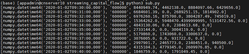
3.6 Subscribe to Real-Time Calculation Results Through Python API
"""
DolphinDB Python API version: 3.0.4.2
Python version: 3.11.9
DolphinDB Server version: 3.00.5
"""
import dolphindb as ddb
import numpy as np
from threading import Event

def resultProcess(lst):
    print(lst)
s = ddb.session()
s.enableStreaming(0)
# 0 means an available port will be selected automatically.
# For DolphinDB Server 1.30.x or versions earlier than 2.00.9, you must specify a port number.
s.subscribe(host="192.xxx.x.140", port=8848, handler=resultProcess, tableName="capitalFlowStream", actionName="SH600000", offset=-1, resub=False, filter=np.array(['600000']))
Event().wait()-
Before you run the Python code, you must first define the stream table capitalFlowStream on the DolphinDB Server and use the
setStreamTableFilterColumnfunction to set its filter column, so that it can work with the filter parameter ofsubscribeprovided by the Python API. -
s.enableStreaming(0): 0 means an available port is automatically selected as the listening port for the client Python process. For DolphinDB Server 1.30.x or versions earlier than 2.00.9, you must specify a port number. -
For the Python API's function
subscribe, the host and port parameters specify the IP address and port of the DolphinDB Server; the handler parameter specifies the callback function, and the sample code defines a user-defined callback functionresultProcessthat prints the data received in real time; the tableName parameter specifies the stream table on the DolphinDB Server, and the sample code subscribes to capitalFlowStream; the offset parameter is set to -1, which means subscribing from the latest record in the stream table; the resub parameter specifies whether to reconnect automatically; and filter specifies the subscription filter condition. In the sample code, it subscribes to the calculation results for 600000 in the SecurityID column of the stream table capitalFlowStream.
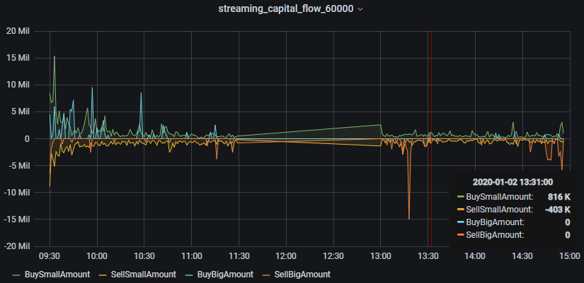
3.7 Monitor Capital Flows in Real Time with Grafana
To configure a DolphinDB data source in Grafana and monitor DolphinDB tables, see Grafana Datasource.
This tutorial monitors the minute-level inflows of small buy orders, small sell orders, large buy orders, and large sell orders.
Query code in Grafana:
-
Capital in small buy orders
select gmtime(TradeTime) as time_sec, BuySmallAmount from capitalFlowStream where SecurityID=`600000 -
Capital in small sell orders (sell-side values are displayed as negative)
select gmtime(TradeTime) as time_sec, -SellSmallAmount as SellSmallAmount from capitalFlowStream where SecurityID=`600000 -
Capital in large buy orders
select gmtime(TradeTime) as time_sec, BuyBigAmount from capitalFlowStream where SecurityID=`600000 -
Capital in large sell orders (sell-side values are displayed as negative)
select gmtime(TradeTime) as time_sec, -SellBigAmount as SellBigAmount from capitalFlowStream where SecurityID=`600000
Grafana displays UTC by default, which may differ from the data timestamp in
the DolphinDB Server depending on the server’s local time zone. Therefore,
the query in Grafana must use the gmtime function for time
zone conversion.
3.8 Replay Historical Data
t = select * from loadTable("dfs://trade", "trade") where time(TradeTime) between 09:30:00.000: 14:57:00.000 order by TradeTime, SecurityID
submitJob("replay_trade", "trade", replay{t, tradeOriginalStream, `TradeTime, `TradeTime, 100000, true, 1})
getRecentJobs()
After execution, the function returns the following information:

If endTime and errorMsg are empty, the task is running normally.
3.9 Functions for Monitoring Stream Processing
-
Query stream table subscription status
getStreamingStat().pubTablesAfter stream tables are subscribed to successfully, you can use the monitoring function to view the detailed subscription information. After execution, the function returns the following information:
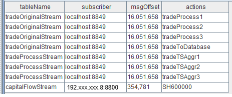
Figure 4. Figure 3-2 Stream Table Subscription Status -
When the subscriber is localhost:8849, it indicates an internal subscription within the node. 8849 is the value of the subPort parameter in the
dolphindb.cfgfile. -
When the subscriber is 192.xxx.xxx.8:8800, it indicates a subscription initiated through the Python API. 8800 is the listening port specified in the Python code.
-
Query the stream table publish queue
getStreamingStat().pubConnsWhen producers generate data and write it to stream tables in real time, you can use the monitoring function to track congestion in the publish queue in real time. After execution, the function returns the following information:
When monitoring publish queue congestion in real time, the key metric to watch is queueDepth, which is the publish queue depth. If the queue depth continues to increase, it indicates that the real-time data volume produced upstream is too high and has exceeded the maximum publishing capacity. As a result, the publish queue becomes congested and real-time calculation latency increases.
queueDepthLimit is the value of the maxPubQueueDepthPerSite parameter in the
dolphindb.cfgfile. It specifies the maximum depth of the message queue on the publishing node, measured in records. -
Query the internal subscriber's consumption status
getStreamingStat().subWorkersAfter the stream table publishes producer data received in real time to internal subscribers on the node, you can use the monitoring function to track congestion in the consumption queue in real time. After execution, the function returns the following information:
When monitoring consumption queue congestion in real time, the key metric to watch is queueDepth of each subscription, which is the consumption queue depth. If the consumption queue depth for a subscription continues to increase, it indicates that the subscription's consumer processing thread has exceeded its maximum capacity. This causes congestion in the consumption queue and increases real-time calculation latency.
queueDepthLimit is the value of the maxSubQueueDepthPerSite parameter in the
dolphindb.cfgfile. It specifies the maximum depth of the message queue on the subscriber node, measured in records.
4. Results Display
This chapter shows how real-time calculation results are presented in different scenarios, including querying result tables within a DolphinDB node, subscribing in real time through the Python API, and visualizing and monitoring results in Grafana.
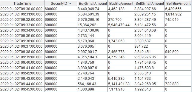
4.1 Result Tables Within the Node
You can query the result table capitalFlowStream in real time through any DolphinDB API, or view its results in real time in the DolphinDB GUI. The output is as follows:
4.2 Real-Time Results Subscribed Through the Python API
4.3 Real-Time Monitoring Results in Grafana
5. Appendix
This chapter provides the complete materials used in the tutorial, including the project code and sample data.