FICC Curve and Surface Builder

1. Introduction

Constructing yield curves and option volatility surfaces is a critical component of financial engineering and quantitative analysis. It ensures pricing accuracy and consistency, and provides a solid foundation for subsequent risk management and trading decisions. Even a minor error in curve construction can lead to pricing deviations or risk misjudgments amounting to millions or even billions.

As markets evolve (e.g., the transition from LIBOR to SOFR) and products become more complex (e.g., structured products like Snowball), the models and techniques for building curves and surfaces have become increasingly complex and important.

DolphinDB V3.00.4 introduces four construction functions for market data curves and surfaces:


Function Name	Model	Description
bondYieldCurveBuilder	Bootstrap/NS/NSS	Builds bond yield curve
irSingleCurrencyCurveBuilder	Bootstrap	Builds single-currency interest rate swap curve
irCrossCurrencyCurveBuilder	Bootstrap	Builds cross-currency interest rate swap curve (implied foreign currencies interest rate curve)
fxVolatilitySurfaceBuilder	SVI/SABR/Linear/CubicSpline	Builds FX Option Volatility Surface

The following sections provide detailed descriptions of these four functions.

2. bondYieldCurveBuilder

The spot curve (zero-coupon yield curve) is crucial for bond pricing and risk management. Its shape (steep, flat, or inverted) and expected changes form the foundation for various trading strategies. This section introduces the method for building a bond yield curve (deriving spot rates from yield to maturity).

2.1 Bootstrap

Bootstrapping is a core and classic financial engineering method used to derive the spot rate curve from a series of market-traded, arbitrage-free bond prices. The method starts with the bond having the shortest residual maturity. Using its yield to maturity (YTM), the bond's dirty price is calculated via bondCalculator. Next, we use an assumed spot curve to price the bond and obtain the bond's net present value (NPV). The spot rate is then adjusted iteratively until the NPV matches the dirty price (with a small error margin). This process determines the spot rate corresponding to the bond's maturity, and by repeating this for all bonds, the entire spot rate curve is derived.

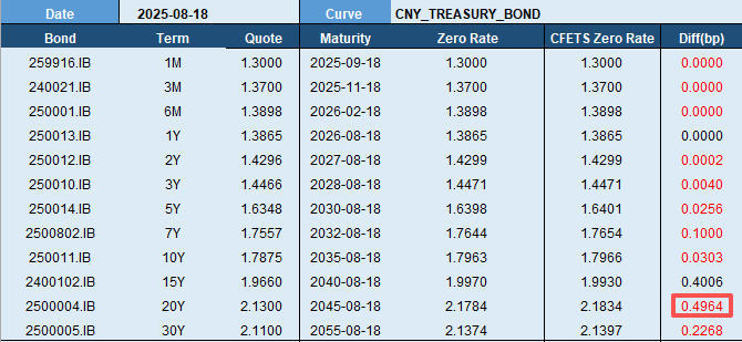
For this example, we refer to the benchmark bond list for the August 2025 national bond yield curve, provided by China Foreign Exchange Trade System (CFETS). Using the closing data from August 18, 2025, we applied bootstrapping to obtain the spot curve (“Zero Rate” column). By comparing this with the CFETS spot curve (“CFETS Zero Rate” column), the maximum error was found at the Term of 20Y, with an error of 0.4964 basis points. Errors for all other maturities were less than 0.5 bp.

2.2 Nelson-Siegel (NS)

Introduced by Nelson and Siegel (1987), the Nelson-Siegel (NS) model is widely used to analyze the bond yield curve. It uses four parameters with distinct economic significance to describe the variations of the yield curve under varying market conditions.

The NS model defines the instantaneous forward rate as:

The model has four parameters: β₀, β₁, β₂, and λ, where τ=T-t represents the time to maturity, and λ>0.

The instantaneous forward rate f(t, T) consists of three terms:

The first term, β₀, is the forward rate as τ→∞, so β₀= f(∞).
The second term is a monotonic function that decreases when β₁> 0 and increases when β₁ < 0.
The third term is a non-monotonic function that generates a hump in the curve.

When τ→0, the second term approaches β₁, and the third term approaches zero. Therefore f(0) = β₀ + β₁.

Integrating the instantaneous forward rate derives the formula for the spot rate: (Formula 1)

Parameter interpretations:

β₀ (Level): Its loading is constant, affecting all terms equally. Therefore, β₀ controls the overall rate level; changes in β₀ cause the entire curve to shift up or down.
β₁ (Slope): Its loading decreases monotonically from 1 to 0, primarily impacting short-term rates. Thus, β₁ controls the slope and steepness of the curve.
β₂ (Curvature): Its loading is hump-shaped, rising from 0 to 1 and then falling back to 0. β₂ mainly affects mid-term rates and thus controls the curvature of the curve.
λ (Decay): It represents the decay speed of the factor loadings for β₁ and β₂, with larger values indicating faster decay.

To build spot curve using the NS model, we first calculate the dirty price of each sample bond based on its YTM via bondCalculator. Then, the assumed spot rate (Formula 1) is used as the discount curve to price the bond and calculate its NPV. For n sample bonds, we can obtain n pairs of (dirty, NPV).

The four parameters are obtained by minimizing the following objective function:

2.3 Nelson-Siegel-Svensson (NSS)

The NSS model (Svensson, 1994) extends the NS model by adding two additional parameters to better simulate a second hump-shaped curve. The NSS model defines the instantaneous forward rate as:

Integrating the instantaneous forward rate derives the spot rate:

The NSS model follows the same construction process as the NS model, but with a different spot rate formula.

2.4 Example

// Taking the construction of the China bond yield curve on August 18, 2025, as an example
bond1 = {
    "productType": "Cash",
    "assetType": "Bond",
    "bondType": "DiscountBond",
    "instrumentId": "259916.IB",
    "start": 2025.03.13,
    "maturity": 2025.09.11,
    "issuePrice":  99.2070,
    "dayCountConvention": "ActualActualISDA"
}
bond2 = {
    "productType": "Cash",
    "assetType": "Bond",
    "bondType": "FixedRateBond",
    "instrumentId": "240021.IB",
    "start": 2024.10.25,
    "maturity": 2025.10.25,
    "coupon": 0.0133,
    "frequency": "Annual",
    "dayCountConvention": "ActualActualISDA"
}
bond3 = {
    "productType": "Cash",
    "assetType": "Bond",
    "bondType": "FixedRateBond",
    "instrumentId": "250001.IB",
    "start": 2025.01.15,
    "maturity": 2026.01.15,
    "coupon": 0.0116,
    "frequency": "Annual",
    "dayCountConvention": "ActualActualISDA"
}
bond4 = {
    "productType": "Cash",
    "assetType": "Bond",
    "bondType": "FixedRateBond",
    "instrumentId": "250013.IB",
    "start": 2025.07.25,
    "maturity": 2026.07.25,
    "coupon": 0.0133,
    "frequency": "Annual",
    "dayCountConvention": "ActualActualISDA"
}
bond5 = {
    "productType": "Cash",
    "assetType": "Bond",
    "bondType": "FixedRateBond",
    "instrumentId": "250012.IB",
    "start": 2025.06.15,
    "maturity": 2027.06.15,
    "coupon": 0.0138,
    "frequency": "Annual",
    "dayCountConvention": "ActualActualISDA"
}
bond6 = {
    "productType": "Cash",
    "assetType": "Bond",
    "bondType": "FixedRateBond",
    "instrumentId": "250010.IB",
    "start": 2025.05.25,
    "maturity": 2028.05.25,
    "coupon": 0.0146,
    "frequency": "Annual",
    "dayCountConvention": "ActualActualISDA"
}

referenceDate = 2025.08.18
bondsTmp = [bond1, bond2, bond3, bond4, bond5, bond6]
bonds = parseInstrument(bondsTmp)
/*
This case references CFETS, using standard maturities. The residual maturities (term) and quotes (quote) for each sample bond are simulated
https://www.chinamoney.com.cn/english/bmkycvcyccyccychdt/index.html
*/
terms = [1M, 3M, 6M, 1y, 2y, 3y]
quotes=[1.3000, 1.3700, 1.3898, 1.3865, 1.4296, 1.4466]/100
       
// method = "BoostStarp"
bootstrapCurve = bondYieldCurveBuilder(referenceDate, `CNY, bonds, terms, quotes, "ActualActualISDA", method='Bootstrap')
bootstrapCurveDict = extractMktData(bootstrapCurve)
print(bootstrapCurveDict)

// method = "NS"
nsCurve = bondYieldCurveBuilder(referenceDate, `CNY, bonds, terms, quotes, "ActualActualISDA", method='NS')
nsCurveDict = extractMktData(nsCurve)
print(nsCurveDict)

// method = "NSS"
nssCurve = bondYieldCurveBuilder(referenceDate, `CNY, bonds, terms, quotes, "ActualActualISDA", method='NSS')
nssCurveDict=extractMktData(nssCurve)
print(nssCurveDict)

3. irSingleCurrencyCurveBuilder

Interest rate swaps (IRS) are important financial derivatives that allow two parties to exchange interest cash flows based on the same nominal principal, but with different interest rate calculation methods over a specified period. Typically, they involve exchanging fixed and floating interest rates, but without exchanging the principal. The pricing of IRS requires the use of an IRS curve. This section introduces the construction of a single-currency IRS curve, involving the following financial instruments:

Deposit Rates (Depo): Provide short-term interest rate information (e.g., 1 day to 1 Y).
Forward Rate Agreements (FRA): Provide forward rates for short to medium term (e.g., 3M to 6M).
Interest Rate Futures (Futures): Provide implied forward rates for the short to medium term (e.g., 3M to 2Y).
Interest Rate Swaps (Swaps): Provide fixed interest rates for the medium to long term (e.g., 1Y to 30Y).

3.1 Bootstrap

For the Chinese market, we selected Depo and Swaps as instruments and apply bootstrapping for curve construction (refer to [1]). The following images show the construction results for the CNY_FR_007 and CNY_SHIBOR_3M curves.

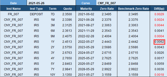
Taking the market data from May 26, 2021, we used the quotes for each maturity of CNY_FR_007 (shown in the “Quote” column) and applied Bootstrapping to derive the spot curve (shown in the “Zero Rate” column). Comparing it to the spot curve from another large institution (shown in the “Benchmark Zero Rate” column), the error was nearly zero.

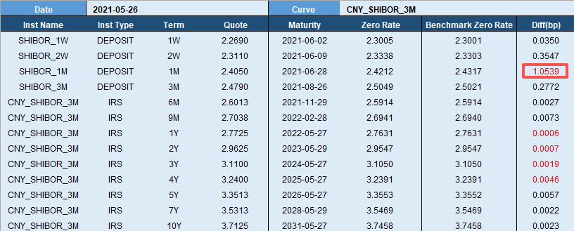
Similarly, for the CNY_SHIBOR_3M curve, using the quotes for each maturity (in the “Quote” column), we applied bootstrapping to derive the spot curve (in the “Zero Rate” column). When compared to the spot curve from another large institution (in the “Benchmark Zero Rate” column), the maximum error was 1.0539 bp, with errors for other maturities all less than 0.5 bp.

3.2 Examples

Example 1. Build an IRS curve denominated in CNY, referenced to the FR_007 floating rate.

referenceDate = 2021.05.26
currency = "CNY"
terms = [7d, 1M, 3M, 6M, 9M, 1y, 2y, 3y, 4y, 5y, 7y, 10y]
instNames = take("CNY_FR_007", size(terms))
instNames[0] = "FR_007"
instTypes = take("IrVanillaSwap", size(terms))
instTypes[0] = "Deposit"
quotes = [2.3500, 2.3396, 2.3125, 2.3613, 2.4075, 2.4513, 2.5750, 2.6763, 2.7650, 2.8463, 2.9841, 3.1350]\100
dayCountConvention = "Actual365"
curve = irSingleCurrencyCurveBuilder(referenceDate, currency, instNames, instTypes, terms, quotes, dayCountConvention, curveName="CNY_FR_007")
curveDict = extractMktData(curve)
print(curveDict)

Example 2. Build an IRS curve denominated in CNY, referenced to the SHIBOR_3M floating rate.

referenceDate = 2021.05.26
currency = "CNY"
terms = [1w, 2w, 1M, 3M, 6M, 9M, 1y, 2y, 3y, 4y, 5y, 7y, 10y]
instNames = take("CNY_SHIBOR_3M", size(terms))
instNames[0] = "SHIBOR_1W"
instNames[1] = "SHIBOR_2W"
instNames[2] = "SHIBOR_1M"
instNames[3] = "SHIBOR_3M"
instTypes = take("IrVanillaSwap", size(terms))
instTypes[0] = "Deposit"
instTypes[1] = "Deposit"
instTypes[2] = "Deposit"
instTypes[3] = "Deposit"
quotes = [2.269, 2.311, 2.405, 2.479, 2.6013, 2.7038,2.7725,
          2.9625, 3.11, 3.24, 3.3513, 3.5313, 3.7125]/100
dayCountConvention = "Actual365"
curve = irSingleCurrencyCurveBuilder(referenceDate, currency, instNames, instTypes, terms, quotes, dayCountConvention)
curveDict = extractMktData(curve)
print(curveDict)

4. irCrossCurrencyCurveBuilder

In pricing FX products, spot curves for both currencies are required to reflect their respective funding costs. This makes the construction of the implied foreign currencies interest rate curve essential. Commonly used instruments include:

FX Swaps (FxSwap): Provide short-term interest rate information.
Cross-Currency Swaps (CrossCurrencySwap): Provide interest rate for medium to long term.

4.1 Bootstrap

For the Chinese market, we use FxSwap and FX spot quotes, and derive the implied foreign currency interest rate curve using the Interest Rate Parity (IRP) formula. Based on the forward exchange rate formula (with continuous compounding as an example):

Where:

S₁ is the near leg (spot) exchange rate.
S₂ is the far leg (forward) exchange rate.
t is the maturity of the swap.
SwapPoint_t is the quoted FX swap.
r_d,t is the CNY zero-coupon rate for maturity t.
r_f,t is the USD zero-coupon rate for maturity t.

Here is the construction result of the implied USD yield curve (USD_USDCNY_FX):

Using USDCNY market data from August 18, 2025, we applied the IRP formula to derive the USD spot curve (“Zero Rate” column), based on FX swap quotes (“Quote” column), the spot exchange rate, and the CNY spot rate curve (“CNY Zero Rate” column). The resulting “Zero Rate” column closely aligns with the “CFETS Zero Rate”, with errors near zero across all terms.

4.2 Example

// Example of constructing the USDCNY implied yield curve as of August 18, 2025
refDate = 2025.08.18
spotDate1 = temporalAdd(refDate, 2, "XNYS")    //Spot date for USD, where "XNYS" refers to the US trading calendar   
spotDate2 = temporalAdd(refDate, 2, "CFET")   //Spot date for CNY, where "CFET" refers to the China trading calendar   
spotDate = max(spotDate1, spotDate2)
instNames = take("USDCNY", 13)
instTypes = take("FxSwap", 13)
terms = ["1d", "1w", "2w", "3w", "1M", "2M", "3M", "6M", "9M", "1y", "18M", "2y", "3y"]
curveDates = array(DATE)
// Calculate the maturity date for each FX swap quote, serving as the time axis for the curve
for(term in terms){
    dur = duration(term)
    d1 = transFreq(temporalAdd(spotDate, dur), "XNYS", "right", "right")
    d2 = transFreq(temporalAdd(spotDate, dur), "CFET", "right", "right")
    curveDates.append!(max(d1, d2))
 }
quotes = [-5.54, -39.00, -75.40, -113.20, -177.00, -317.00, -466.00, -898.50, 
         -1284.99, -1676.00, -2320.00, -2870.00, -3962.50] \ 10000  // fx swap points

curve = {
    "mktDataType": "Curve",
    "curveType": "IrYieldCurve",
    "referenceDate": refDate,
    "currency": "CNY",
    "dayCountConvention": "Actual365",
    "compounding": "Continuous",
    "interpMethod": "Linear",
    "extrapMethod": "Flat",
    "dates": curveDates,
    "values": [1.5113, 1.5402, 1.5660, 1.5574, 1.5556, 1.5655, 1.5703, 
               1.5934, 1.6040, 1.6020, 1.5928, 1.5842, 1.6068] \ 100,
    "settlement": spotDate
}

cnyShibor3m = parseMktData(curve)

spot = 7.1627
curve = irCrossCurrencyCurveBuilder(refDate, "USD", instNames, instTypes, terms, quotes, "USDCNY", spot, "Actual365", cnyShibor3m, "Continuous")
curveDict = extractMktData(curve)
for(i in 0..(size(quotes)-1) ){
    print(curveDict["values"][i]*100)
}

5. fxVolatilitySurfaceBuilder

FX option pricing requires volatility, which is interpolated from the volatility surface based on the option's strike price and residual maturity.

Unlike other assets where options are quoted in terms of strike-vol, FX options are quoted in terms of delta-vol. Therefore, the first step in constructing the volatility surface is to convert delta into strike. The conversion process is as follows:

//Step1: Calculate the volatility for individual options
sigma_25c = sigma_atm + bf_25 + 0.5 * rr_25   //Volatility for delta = 0.25 call
sigma_25p = sigma_atm + bf_25 - 0.5 * rr_25   //Volatility for delta =-0.25 put
sigma_10c = sigma_atm + bf_10 + 0.5 * rr_10   //Volatility for delta = 0.10 call
sigma_10p = sigma_atm + bf_10 - 0.5 * rr_10   //Volatility for delta = -0.10 put
/*
Where:
sigma_atm: The volatility for at-the-money options
bf_25: The butterfly option quote for delta = 0.25  
rr_25: The risk reversal (RR) option quote for delta = 0.25  
bf_10: The butterfly option quote for delta = 0.10  
rr_10: The risk reversal (RR) option quote for delta = 0.10 
*/

//Step2: Use the Black-Scholes formula to reverse calculate the strike price for delta. The calculation is not detailed here, but you can refer to the formula in [3] for further information

After obtaining the strike-vol (smile) data point, the volatility smile can be constructed using the following models. While simpler methods like Linear and CubicSpile interpolation are not detailed here, this section focuses on the SVI and SABR models.

5.1 SVI (Stochastic Volatility Inspired)

The SVI model, proposed by Jim Gatheral, models the implied volatility smile using total variance: (Formula 2)

Where:

ω(k): Total variance, defined as ω(k)=σ²_imp×T, where σ²_imp is the implied volatility and T is the maturity date.
k: Log moneyness, defined as k=ln(K/F), where K is the strike price and F is the forward exchange rate.
a: Minimum total variance, which controls the baseline level of total variance.
b: The slope of the total variance.
ρ: The symmetry of the smile (ρ∈[-1,1]), typically negative.
m: The center of the log moneyness.
σ: The width of the smile.

ω(k) in Formula 2 can be obtained from strike-vol in the previous section. The strike is the K in k=ln(K/F) (where F can be calculated using the forward exchange rate formula), and vol is the implied volatility σ_imp. The objective function is defined as

and can be minimized using algorithms like Levenberg-Marquardt to solve for the five parameters, allowing us to obtain the volatility for any strike on the entire smile curve.

5.2 SABR (Stochastic Alpha Beta Rho)

The SABR model provides an analytical approximation for the implied volatility:

Where:

IV(K): The implied volatility for a given strike price K.
α: Initial volatility, which controls the volatility level.
β: Controls the sensitivity of volatility to the underlying asset's price (typically 0≤β≤1).
ρ: The correlation between the underlying asset price and volatility.
υ: Volatility of volatility (vol-of-vol).
K: Strike price.
F: Forward exchange rate.
T: Maturity date.

The objective function is defined as

and can be minimized using algorithms like Levenberg-Marquardt to solve for the four parameters, allowing us to obtain the volatility for any strike on the entire smile curve.

5.3 Example

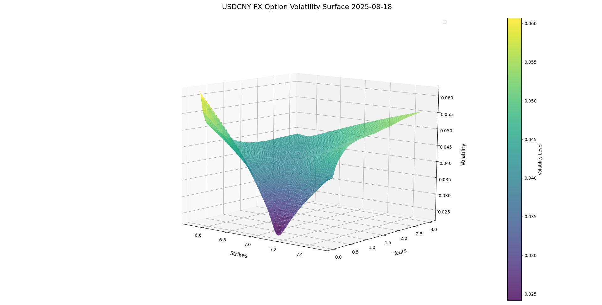
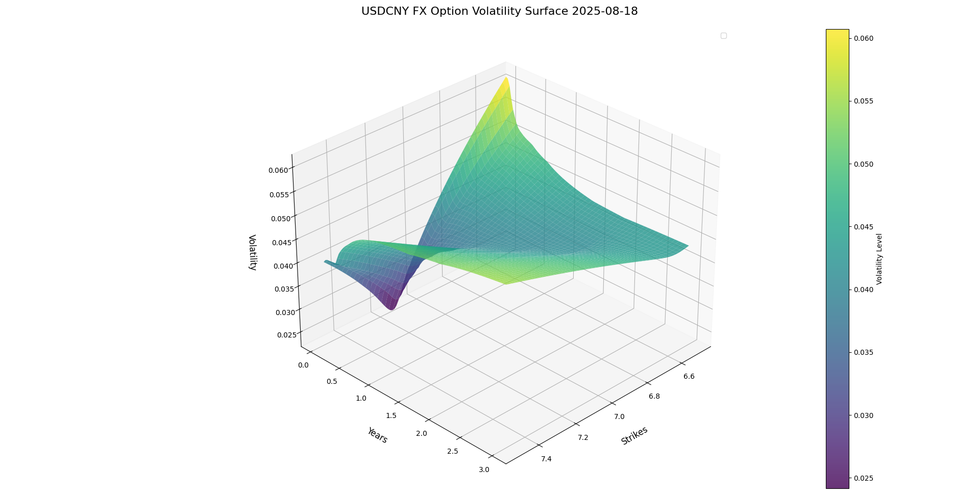
Using CFETS data for August 18, 2025, we selected the USDCNY FX option delta quote matrix as parameters. The SVI model was applied to fit the volatility smile, generating an FX volatility surface for pricing FX options.

refDate = 2025.08.18
ccyPair = "USDCNY"
quoteTerms = ['1d', '1w', '2w', '3w', '1M', '2M', '3M', '6M', '9M', '1y', '18M', '2y', '3y']
quoteNames = ["ATM", "D25_RR", "D25_BF", "D10_RR", "D10_BF"]
quotes = [0.030000, -0.007500, 0.003500, -0.010000, 0.005500, 
          0.020833, -0.004500, 0.002000, -0.006000, 0.003800, 
          0.022000, -0.003500, 0.002000, -0.004500, 0.004100, 
          0.022350, -0.003500, 0.002000, -0.004500, 0.004150, 
          0.024178, -0.003000, 0.002200, -0.004750, 0.005500, 
          0.027484, -0.002650, 0.002220, -0.004000, 0.005650, 
          0.030479, -0.002500, 0.002400, -0.003500, 0.005750, 
          0.035752, -0.000500, 0.002750,  0.000000, 0.006950, 
          0.038108,  0.001000, 0.002800,  0.003000, 0.007550, 
          0.039492,  0.002250, 0.002950,  0.005000, 0.007550, 
          0.040500,  0.004000, 0.003100,  0.007000, 0.007850, 
          0.041750,  0.005250, 0.003350,  0.008000, 0.008400, 
          0.044750,  0.006250, 0.003400,  0.009000, 0.008550]
quotes = reshape(quotes, size(quoteNames):size(quoteTerms)).transpose()
spot = 7.1627
curveDates = [2025.08.21, 2025.08.27, 2025.09.03, 2025.09.10, 2025.09.22, 2025.10.20,
  2025.11.20, 2026.02.24,2026.05.20, 2026.08.20, 2027.02.22, 2027.08.20, 2028.08.21]
domesticCurveInfo = {
    "mktDataType": "Curve",
    "curveType": "IrYieldCurve",
    "referenceDate": refDate,
    "currency": "CNY",
    "dayCountConvention": "Actual365",
    "compounding": "Continuous",  
    "interpMethod": "Linear",
    "extrapMethod": "Flat",
    "frequency": "Annual",
    "dates": curveDates,
    "values":[1.5113, 1.5402, 1.5660, 1.5574, 1.5556, 1.5655, 1.5703, 
              1.5934, 1.6040, 1.6020, 1.5928, 1.5842, 1.6068]/100
}
foreignCurveInfo = {
    "mktDataType": "Curve",
    "curveType": "IrYieldCurve",
    "referenceDate": refDate,
    "currency": "USD",
    "dayCountConvention": "Actual365",
    "compounding": "Continuous",  
    "interpMethod": "Linear",
    "extrapMethod": "Flat",
    "frequency": "Annual",
    "dates": curveDates,
    "values":[4.3345, 4.3801, 4.3119, 4.3065, 4.2922, 4.2196, 4.1599, 
              4.0443, 4.0244, 3.9698, 3.7740, 3.6289, 3.5003]/100
}
domesticCurve = parseMktData(domesticCurveInfo)
foreignCurve = parseMktData(foreignCurveInfo)
surf = fxVolatilitySurfaceBuilder(refDate, ccyPair, quoteNames, quoteTerms, quotes, spot, domesticCurve, foreignCurve)
surfDict = extractMktData(surf)
print(surfDict)

6. Utility Functions

6.1 curvePredict

After the curve is constructed, we can use the curvePredict function to retrieve the curve value for any given date.

curveDict = {
    "mktDataType": "Curve",
    "curveType": "IrYieldCurve",
    "referenceDate": 2025.08.18,
    "currency": "CNY",
    "dayCountConvention": "ActualActualISDA",
    "compounding": "Continuous",  
    "interpMethod": "Linear",
    "extrapMethod": "Flat",
    "frequency": "Annual",
    "dates": [2025.08.21, 2025.08.27, 2025.09.03, 2025.09.10, 2025.09.22, 2025.10.20,
     2025.11.20, 2026.02.24, 2026.05.20, 2026.08.20, 2027.02.22,2027.08.20, 2028.08.21],
    "values":[1.5113, 1.5402, 1.5660, 1.5574, 1.5556, 1.5655, 1.5703, 
              1.5934, 1.6040, 1.6020, 1.5928, 1.5842, 1.6068]/100
}

curve = parseMktData(curveDict)
curvePredict(curve, 2025.10.18)
// output: 0.0156
curvePredict(curve, 1.0)
// output: 0.0160
curvePredict(curve, [2025.10.18, 2026.10.18])
// output: [0.0156,0.0159]
curvePredict(curve, [1.0, 2.0])
// output: [0.0160,0.0158]

6.2 optionVolPredict

The volatility surface is a 3D surface. We can use the optionVolPredict function to retrieve the volatility for specified dates and strike prices.

refDate = 2025.08.18
ccyPair = "USDCNY"
quoteTerms = ['1d', '1w', '2w', '3w', '1M', '2M', '3M', '6M', '9M', '1y', '18M', '2y', '3y']
quoteNames = ["ATM", "D25_RR", "D25_BF", "D10_RR", "D10_BF"]
quotes = [0.030000, -0.007500, 0.003500, -0.010000, 0.005500, 
          0.020833, -0.004500, 0.002000, -0.006000, 0.003800, 
          0.022000, -0.003500, 0.002000, -0.004500, 0.004100, 
          0.022350, -0.003500, 0.002000, -0.004500, 0.004150, 
          0.024178, -0.003000, 0.002200, -0.004750, 0.005500, 
          0.027484, -0.002650, 0.002220, -0.004000, 0.005650, 
          0.030479, -0.002500, 0.002400, -0.003500, 0.005750, 
          0.035752, -0.000500, 0.002750,  0.000000, 0.006950, 
          0.038108,  0.001000, 0.002800,  0.003000, 0.007550, 
          0.039492,  0.002250, 0.002950,  0.005000, 0.007550, 
          0.040500,  0.004000, 0.003100,  0.007000, 0.007850, 
          0.041750,  0.005250, 0.003350,  0.008000, 0.008400, 
          0.044750,  0.006250, 0.003400,  0.009000, 0.008550]

quotes = reshape(quotes, size(quoteNames):size(quoteTerms)).transpose()

spot = 7.1627
curveDates = [2025.08.21, 2025.08.27, 2025.09.03, 2025.09.10, 2025.09.22, 2025.10.20,
  2025.11.20, 2026.02.24, 2026.05.20, 2026.08.20, 2027.02.22, 2027.08.20, 2028.08.21]

domesticCurveInfo = {
    "mktDataType": "Curve",
    "curveType": "IrYieldCurve",
    "referenceDate": refDate,
    "currency": "CNY",
    "dayCountConvention": "Actual365",
    "compounding": "Continuous",  
    "interpMethod": "Linear",
    "extrapMethod": "Flat",
    "frequency": "Annual",
    "dates": curveDates,
    "values":[1.5113, 1.5402, 1.5660, 1.5574, 1.5556, 1.5655, 1.5703, 
              1.5934, 1.6040, 1.6020, 1.5928, 1.5842, 1.6068]/100
}
foreignCurveInfo = {
    "mktDataType": "Curve",
    "curveType": "IrYieldCurve",
    "referenceDate": refDate,
    "currency": "USD",
    "dayCountConvention": "Actual365",
    "compounding": "Continuous",  
    "interpMethod": "Linear",
    "extrapMethod": "Flat",
    "frequency": "Annual",
    "dates": curveDates,
    "values":[4.3345, 4.3801, 4.3119, 4.3065, 4.2922, 4.2196, 4.1599, 
              4.0443, 4.0244, 3.9698, 3.7740, 3.6289, 3.5003]/100
}

domesticCurve = parseMktData(domesticCurveInfo)
foreignCurve = parseMktData(foreignCurveInfo)

surf = fxVolatilitySurfaceBuilder(refDate, ccyPair, quoteNames, quoteTerms, quotes, spot, domesticCurve, foreignCurve)

optionVolPredict(surf, 2025.10.18, 7)
/* output:
           7                
           -----------------
2025.10.18|0.035427722673281
*/
optionVolPredict(surf, 2025.10.18, [7.1,7.2])
/* output:
           7.1               7.2
           ----------------- -----------------
2025.10.18|0.029466799513362 0.029268084254983
*/
optionVolPredict(surf, [2025.10.18, 2026.10.18], 7)
/* output:
           7                
           -----------------
2025.10.18|0.035427722673281
2026.10.18|0.040453528763062
*/
optionVolPredict(surf, [2025.10.18, 2026.10.18], [7.1, 7.2])
/* output:
           7.1               7.2
           ----------------- -----------------
2025.10.18|0.029466799513362 0.029268084254983
2026.10.18|0.042188693924168 0.044408563755123
*/

7. Summary and Outlook

This tutorial demonstrates the theory and methods for constructing interest rate curves and FX option volatility surfaces. It also provides detailed usage instructions for DolphinDB’s built-in functions, compares the results with relevant benchmarks, and offers utility functions for user convenience.

In the future, we will continue to iterate and update in two areas:

Diversifying construction functions: We plan to introduce new builders to cover more curves and surfaces, such as commodity forward curves, Credit Default Swap (CDS) curves, commodity future/option volatility surfaces, etc.
Broadening assets coverage: We plan to expand existing functions to support more underlying assets. For example, irSingleCurrencyCurveBuilder currently supports only CNY_FR_007 and CNY_SHIBOR_3M, but future updates will support curves like USD_SOFR and EUR_ESTR.

The construction of yield curves and volatility surfaces is a core function of financial engineering. These intermediate market data not only serve as the basis for pricing and risk control, but also provide essential support for numerous quantitative strategies. Looking ahead, we will keep pace with the market and innovate to offer more financial engineering functions for our clients. Stay tuned!

References

[1] F. Ametrano and M. Bianchetti. Everything you always wanted to know about Multiple Interest Rate Curve Bootstrapping but were afraid to ask (April 2, 2013). Available at SSRN: Everything You Always Wanted to Know About Multiple Interest Rate Curve Bootstrapping but Were Afraid to Ask or Everything You Always Wanted to Know About Multiple Interest Rate Curve Bootstrapping but Were Afraid to Ask, 2013.

[2] Reiswich, D., & Wystup, U. (2010). FX Volatility Smile Construction. CPQF Working Paper Series, No. 20. Frankfurt School of Finance & Management.

[3] Clark, I. J. (2011). Foreign exchange option pricing: A practitioner's guide. Chichester, West Sussex, PO19 8SQ, United Kingdom: John Wiley & Sons Ltd.

Appendix

curve_volsurf_builder.dos