DolphinDB-Based Solution for Quantitative Cryptocurrency Trading
1. Overview
In recent years, the global cryptocurrency market has grown rapidly. The proliferation of exchanges and cryptocurrency types, round-the-clock trading, massive trading volumes, and high price volatility have created unprecedented opportunities for quantitative cryptocurrency trading firms. At the same time, the complexity of the cryptocurrency market brings significant technical challenges. First, data sources are highly scattered and data structures are complex, leading to high costs for data ingestion and management. Second, high-frequency trading generates massive volumes of data, placing extremely high demands on database performance. Third, the separation between strategy research and live trading systems makes it difficult to directly apply research findings to live trading. Against this backdrop, building a high-performance, low-latency, and scalable integrated quantitative trading platform has become a core competitive advantage for quantitative cryptocurrency trading firms.
Tailored to the cryptocurrency market, DolphinDB delivers an end-to-end trading solution that combines high-performance distributed storage and computing, low-latency streaming processing, backtesting, and order matching. The solution covers the full workflow from data storage and processing to strategy development and live trading, helping trading firms accelerate strategy development and validation. Key features of the solution include:
- Comprehensive solution for ingesting and storing market data from Binance and OKX, along with a monitoring and alerting mechanism that significantly reduces data maintenance costs.
- Built-in data cleansing and processing functions that eliminate tedious preprocessing steps, lower the barrier to strategy development, and accelerate strategy implementation.
- Batch and streaming factor computation, integrated with Python-based training models to generate factor signals in real time.
- A live trading module with the same usage as the DolphinDB backtesting plugin, allowing high-performing strategies to be directly deployed in live trading.
In addition, the solution includes real-time risk control models for key risk metrics, enabling real-time monitoring and alerting of account risk to help manage risk effectively. It also extends to features such as strategy code management and user management.
Version requirements: We recommend that you use DolphinDB Server 3.00.4 to implement the solution.
1.1 Market Data Processing
In quantitative trading research, market data is the core for strategy development, factor construction, backtesting, simulated trading, and live trading. DolphinDB integrates a high-performance distributed storage engine with a streaming computation framework, enabling efficient storage and batch processing of massive data while also supporting real-time computation and persistence of streaming data. The processing workflow for cryptocurrency market data is divided into three parts: data ingestion, computation, and consumption.
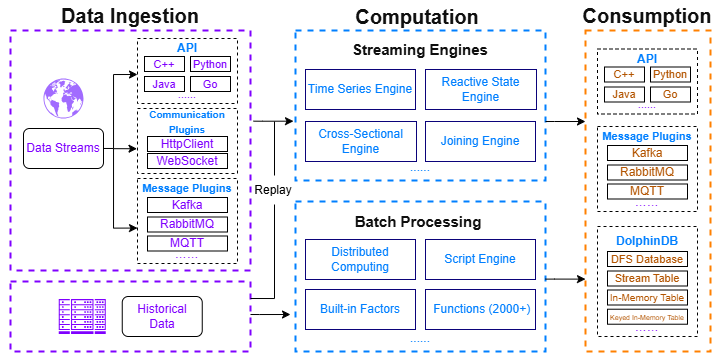
Data ingestion: This solution integrates data sources from two major cryptocurrency exchanges—Binance and OKX. For different data types, it provides best-practice database and table designs, covering tick data, trading data, OHLC data, funding rate data, liquidation data, and more (see Chapter 2 for details). In addition, it supports customizing the cryptocurrency list to meet diverse data requirements. DolphinDB supports acquiring trading data through the following tools:
- APIs: APIs for multiple programming languages, including Python, C++, Java, and Go.
- Plugins: Data communication plugins such as httpClient and WebSocket.
To address issues such as network interruptions, exchange API errors, and database errors, this solution provides a comprehensive monitoring, alerting, and data backfill mechanism to prevent data loss. The specific methods include:
- Writing real-time streaming data to stream tables on two servers simultaneously, with key-based deduplication to mitigate the impact of network disruptions.
- Automatically retrying connections upon abnormal disconnections, caching data locally, and reloading them into the database once the connection is restored.
- Periodically monitoring the status of stream tables and databases, and triggering alerts promptly when anomalies are detected.
- Periodically validating the completeness of OHLC data for the previous trading day and re-fetching missing data when necessary.
Computation: DolphinDB provides a powerful computation framework that supports both batch and streaming processing, including real-time snapshot aggregation, batch and real-time factor computation, and real-time data storage into databases.
- Streaming engines: DolphinDB provides multiple built-in streaming engines, such as the time-series engine (e.g., used to generate OHLC bars at different frequencies), the reactive state engine (e.g., used to cleanse data in real time), join engines (e.g., used to aggregate snapshot data), and the cross-sectional engine (e.g., used to rank cryptocurrency types).
- High-performance batch processing: DolphinDB supports distributed batch processing and comes with multiple factor libraries and more than 2,000 optimized functions. Its powerful programming language enables efficient processing and analysis of large-scale datasets.
Consumption: Results computed by DolphinDB can be stored in DFS tables, in-memory tables, or stream tables. Consumers can subscribe to stream tables in real time to obtain the latest market data for simulated or live trading. Alternatively, computation results can be accessed in real time through APIs or pushed via message middleware.
1.2 Unified Stream and Batch Processing
In quantitative trading research, factor research is a critical part of strategy development. Factors are quantitative metrics that capture market characteristics and reflect price dynamics and risk structures, forming the foundation of model prediction and signal generation.
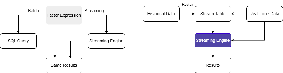
Traditional quantitative research platforms often adopt a dual-system architecture: using scripting languages like Python for strategy and factor development, and high-performance languages such as C++ for real-time computation in production. This approach not only incurs high development and maintenance costs, but also risks inconsistencies between batch and streaming results.
DolphinDB’s unified stream and batch processing framework eliminates this issue by enabling a single codebase that allows seamless migration of factor logic from development to real-time computation. This ensures consistent results between research and live trading while significantly reducing development costs and maintenance complexity.
Based on DolphinDB’s built-in 191 Alpha and WorldQuant 101 Alpha factor libraries, this solution supports both batch and streaming computations for these factors, along with a highly extensible factor storage architecture. User-defined factors can also be developed as needed.
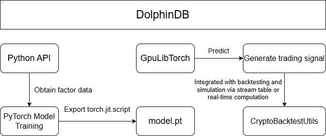
On this foundation, machine learning models, such as LSTM, XGBoost, and Transformer, are trained on existing factors in a Python environment, with full support for data access, preprocessing, and model training. Trained models can be loaded into DolphinDB via the GpuLibTorch plugin for backtesting and simulated trading, enabling real-time trading signal generation. Leveraging these capabilities, this solution delivers an end-to-end pipeline from factor development and streaming-batch computation, to Python-based model training and real-time trading signal generation.
1.3 Backtesting and Simulated Trading
Before being deployed in live trading, quantitative strategies are subjected to extensive backtesting and simulation to validate their effectiveness and feasibility. DolphinDB provides a comprehensive backtesting and simulation framework for cryptocurrency quantitative trading, featuring core components such as historical market data replay, real-time data ingestion, an order matching simulator, and a backtesting engine.
- Historical data replay: In simulated trading, quantitative strategies
usually process real-time data in an event-driven manner. To ensure
consistent strategy logic across backtesting and simulated trading,
DolphinDB provides a data replay mechanism that feeds historical market data
into the backtesting engine in strict chronological order, reproducing real
trading conditions.
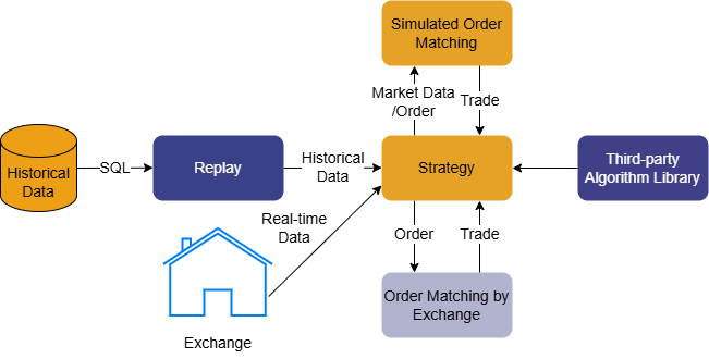
Figure 4. Figure 1-4: Cryptocurrency Backtesting Architecture - Real-time data ingestion: In simulated trading, the DolphinDB backtesting engine supports continuous ingestion of streaming data. During execution, results such as trade details, real-time positions, and account equity are written to stream tables in real time.
- Backtesting plugin: The DolphinDB backtesting plugin includes a built-in order matching simulator optimized to reflect real-world matching logic, enabling more accurate evaluation and prediction of strategy performance in live trading. The plugin consists of four core components: user-defined strategy functions, strategy configuration and creation, market data replay, and execution of the backtesting engine. It supports snapshot and minute-level cryptocurrency market data, as well as multi-account management.

To reduce strategy development costs, we focus on real-world quantitative trading requirements to provide an integrated backtesting and simulation solution. The solution unifies market data replay and processing, backtesting and simulation engine creation, strategy development and code management, strategy visualization and management, and user-level strategy permission control. This allows developers to focus solely on strategy logic, enabling both individual users and quantitative trading teams to conduct efficient research and development with minimal code and a low learning curve.
1.4 Live Trading
After thorough backtesting and simulation, strategy researchers aim to deploy high-performing strategies in live cryptocurrency markets to generate real returns. To support this transition, this solution integrates with exchange order and account APIs and provides a live trading module fully consistent with the simulation logic. This enables a true “single codebase” approach across backtesting, simulation, and live trading. This solution supports both Binance and OKX, offering capabilities such as order placement and cancellation, querying open orders, and retrieving trade details. In addition, it incorporates risk metrics to build real-time risk control models for timely monitoring and alerting of account conditions.
1.5 Real-Time Risk Control
The cryptocurrency market is highly volatile, offering significant return potential alongside substantial risk. In practice, many existing solutions compute risk metrics by directly consuming exchange-provided fields such as margin usage and unrealized profit and loss (P&L). Although simple, this approach has several limitations:
- Risk data provided by exchanges often has low update frequency or high latency, making it difficult to promptly reflect risks caused by rapid market movements.
- It does not support portfolio-level risk computation across multiple accounts.
- It cannot be combined with simulated market data for scenario analysis and stress testing.
To address these issues, we provide a DolphinDB-based real-time risk control solution for cryptocurrency trading. By continuously ingesting exchange account data and periodically computing key metrics such as portfolio’s net asset value, position P&L, total asset value, and leverage ratio, this solution enables timely monitoring and alerting of account risk, helping investors better understand and manage their investment risks. Compared with traditional risk control approaches, this solution offers the following advantages:
- Stronger real-time performance: Compared with exchange-provided leverage estimates, this solution captures market changes promptly and issues real-time risk alerts, ensuring superior timeliness.
- Real-time data persistence: Account information and risk metrics are persisted in real time, enabling advanced analysis, scenario simulation, and stress testing.
- High extensibility: You can flexibly modify and extend risk metric computation to meet diverse risk management requirements across different scenarios.
- Isolation from business logic: The risk control module operates independently from trading logic and runs on read-only account data, ensuring the stability and continuity of the trading system.
2. Historical and Real-Time Data Ingestion
Unlike traditional financial assets, the cryptocurrency market operates with round-the-clock trading, high price volatility, and massive data volumes. These characteristics place much higher demands on database performance, including data storage, querying, and real-time processing. To address these challenges, we leverage DolphinDB’s high-performance storage and computing capabilities to provide a comprehensive solution for data ingestion and storage, data processing, as well as monitoring and data backfill.
This solution integrates two major exchanges (Binance and OKX) as data sources. It supports a wide range of cryptocurrency types and various market data to meet diverse requirements. For certain data types, different modes can be selected (USD-margined, coin-margined, or spot). In addition, this solution implements robust fault-tolerance mechanisms, including automatic reconnection retries, scheduled monitoring, and periodic data backfill, ensuring data completeness and reliability even in scenarios such as network failures or service restarts.
Below is a summary table of all provided market data ingestion scripts, covering both historical and real-time data. The complete data ingestion scripts are included in the Appendix. Exchange-related documentation can be found at: Binance Open Platform and OKX API Guide.
| Data type | Table Type/Name | Script File Name | Description |
|---|---|---|---|
| OHLC data |
|
|
Supports ingesting historical and real-time data to generate OHLC bars at different frequencies.To add new frequencies or modify table names, see Sections 2.2 & 2.3. |
| Tick trade data |
|
|
|
| Aggregated trade data |
|
|
OKX does not provide historical aggregated trade data. |
| Level 2 market data |
|
Real-time data:
|
No historical data. |
| Snapshot market data |
|
Real-time data: depthTradeMergeScript.dos | Merged in real time from level 2 data and aggregated trade data, and persisted in real time. |
| 400-level order book snapshot data |
|
Real-time data: okx_depth_400.py | After retrieving both full and incremental snapshots, the data is processed by the orderbook snapshot engine and persisted in real time. |
| Funding rate data | DFS table: dfs://CryptocurrencyDay/fundingRate |
|
|
| Index price/ mark price OHLC | DFS table:
|
Historical data: historyIndexMarkKLine.py | Not pushed in real time and is retrieved on a scheduled basis, following the funding rate scheduling logic. |
| Metrics data | DFS table: dfs://CryptocurrencyKLine/metrics | Historical data: historyMetrics.py |
|
| Minute-level data for continuous contracts |
|
Real-time data:
|
No historical data. |
| Liquidation data |
|
Real-time data:
|
|
| Trading pair information |
|
Real-time data:
|
No historical data. |
- Binance internally maintains multiple types of historical market data. For details, see Binance Data Collection.
- Instructions for using the historical and real-time data ingestion scripts are provided in Sections 2.2 & 2.3.
2.1 Database and Table Schema
Considering the characteristics of cryptocurrency market data and its usage scenarios, we provide partitioning schemes based on both OLAP and TSDB engines to achieve optimal performance for data ingestion and querying. Taking nine major cryptocurrencies as examples, this section describes the database and table design by combining minute-level OHLC data, tick data, funding rate data, and other datasets. The design supports a certain level of extensibility for additional symbols and is reasonably generic. The database and table creation scripts are provided in the Appendix.
| Database Name | Engine | Partitioning Scheme | Partition Column | Sorting Column | Data Type |
|---|---|---|---|---|---|
| CryptocurrencyTick | TSDB | Daily partition + HASH partition by symbol | Trade time + symbol | Exchange + symbol + trade time |
|
| CryptocurrencyOrderBook | TSDB | Hourly partition + VALUE partition by symbol | Trade time + symbol | Symbol + trade time | High-frequency order book snapshot data (400 levels) |
| CryptocurrencyKLine | OLAP | Yearly partition | Trade time | None |
|
| CryptocurrencyDay | OLAP | 5-year partition | Trade time | None |
|
- For precise database and table design, you need to consider both the data volume of selected cryptocurrencies and their usage scenarios.
- Low-frequency and infrequently queried data, such as funding rate data and liquidation data, are stored in dimension tables.
This solution integrates market data types from both Binance and OKX. For different data types, unified field naming conventions are adopted while preserving exchange-specific fields as much as possible. All timestamp fields are in UTC+0. If any other time zone is used as a reference, the corresponding scripts must be modified for time zone conversion. A complete field description is provided in the Appendix.
2.2 Historical Data Ingestion
This solution provides a complete set of scripts for ingesting historical data, including OHLC data at different frequencies, aggregated trade data, tick trade data, funding rate data, and metrics data. You can specify time ranges, cryptocurrency list, and frequencies (for OHLC data). Historical market data is primarily used for backtesting and data monitoring. Therefore, we recommend that you do not customize database or table names. Otherwise, corresponding table names in scripts need to be modified. In addition, there are differences between the historical data provided by Binance and OKX. Detailed description can be found in the Description column of Table 2-1. The complete historical data ingestion scripts are provided in the Appendix.
2.2.1 Historical Data Ingestion for Binance
Overview
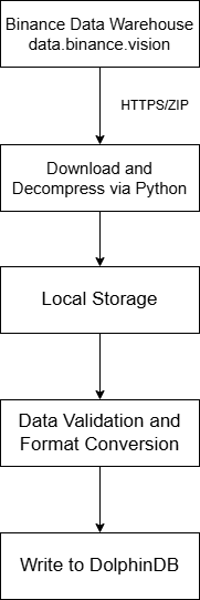
This solution uses Python to batch-download historical data from Binance and import it into DolphinDB. By accessing Binance’s official historical data warehouse, it supports batch processing across multiple trading pairs and date ranges, and includes error handling, logging, and data validation.
- Data source: Access Binance’s official historical data warehouse to view all available assets and the corresponding start dates.
- Data download: Use the requests library to download compressed CSV files, decompress them, and retain the raw data. After successful write, the original files are deleted.
- Data write: Connect to DolphinDB and write the data into the target DFS tables.
- Logging: Record write details, including download status, parsing status, and the number of rows written.
- Workflow control: Support customizing the cryptocurrency list and start/end dates, and automatically iterating over the ingestion workflow.
Core functions
download_file: Downloads the compressed file for a specified date to a given path, decompresses it, removes the .zip file, and returns the CSV file path.parse_csv_to_dataframe: Reads the CSV file, checks for the presence of headers, converts fields to match the required data types for data write, and returns a standardized pandas.DataFrame.import_to_db: Writes the transformed DataFrame into the specified DolphinDB table.process_single_file: Chains the above three functions to process the historical data of a single cryptocurrency for a single day.run: The main control function that iterates in batch over multiple cryptocurrencies and multiple dates, recording overall results.
Variables and usage instructions
Before running, ensure that the target database and tables exist in the DolphinDB server. Modify the following variables according to your requirements and execute the Python program. The Python script is provided in the Appendix.
| Variable | Location | Description |
|---|---|---|
| DDB | config.py | Configures the DolphinDB connection, including host, port, username, and password |
| HIS_CONFIG | config.py | Directory for storing import logs |
| HIS_CONFIG | config.py | Directory for storing downloaded files |
| PROXY | config.py | Proxy address |
| url | In download_file() | URL of the file to download. Adjust as needed;
/futures and /spot
distinguish futures and spot addresses |
| symbols | Configuration parameter | List of symbols for which historical data is downloaded, e.g. ["BTCUSDT"] |
| start_date | Configuration parameter | Start time of the historical data to download |
| end_date | Configuration parameter | End time of the historical data to download |
| db_path | Configuration parameter | Target database path for data import |
| table_name | Configuration parameter | Name of the target DFS table |
| accountType | Configuration parameter | Contract type (varies by data type):
|
| interval | Configuration parameter | OHLC frequency (OHLC data only): '1m', '3m', '5m', '15m', '30m', '1h', '2h', '4h', '6h', '8h', '12h', '1d', '3d', '1w', '1mo' |
| klineType | Configuration parameter | OHLC type (index or mark price only):
|
The following example shows how to import Binance’s historical minute-level OHLC data using historyKline.py. You can reference this example and modify the parameters to import other types of market data.
- Create the required database and tables for the data type. We recommend
that you do not modify table names. For the full script, refer to
createDatabase.dos in the Appendix.
dbName = "dfs://CryptocurrencyKLine" tbName = "minKLine" streamtbName = "Cryptocurrency_minKLineST" db = database(dbName, RANGE, 2010.01M + (0..20)*12) colNames = `eventTime`collectionTime`symbolSource`symbol`open`high`low`close`volume`numberOfTrades`quoteVolume`takerBuyBase`takerBuyQuote`volCcy colTypes = [TIMESTAMP, TIMESTAMP, SYMBOL, SYMBOL, DOUBLE, DOUBLE, DOUBLE, DOUBLE, DOUBLE, INT, DOUBLE, DOUBLE, DOUBLE, DOUBLE] createPartitionedTable(db, table(1:0, colNames, colTypes), tbName, `eventTime) - Install required Python packages such as requests, zipfile, numpy, and dolphindb.
- Modify variables as
needed:
# config.py -- DDB and PROXY must be updated for your setup DDB = {"HOST": '192.xxx.xxx.xx', "PORT": 8848, "USER": 'admin', "PWD": '123456'} BINANCE_BASE_CONFIG = { "PROXY": 'http://127.0.0.1:7890/', "TIMEOUT": 5, "PROBE_COOLDOWN_SECS": 30, "READ_BATCH_SIZE": 20000, "LIVE_GET_TIMEOUT": 0.2 } HIS_CONFIG = {"LOG_DIR": "./logs", "SAVE_DIR": "./data"} # Global settings symbols = ["BTCUSDT","ETHUSDT","ADAUSDT","ALGOUSDT","BNBUSDT","FETUSDT","GRTUSDT","LTCUSDT","XRPUSDT"] start_date = datetime(2025, 8, 11) end_date = datetime(2025, 8, 12) accountType = "um" # Supported: um/cm/spot interval = "1m" # Adjust for different OHLC frequencies db_path = "dfs://CryptocurrencyKLine" table_name = "minKLine" - Execute the Python script to batch-import historical data. Import
progress and results can be monitored via the log files at the custom
LOG_DIR
path.
result = downloader.run(accountType, symbols, klineType, start_date, end_date,
                        interval, db_path, table_name)
2.2.2 Historical Data Ingestion for OKX
Unlike Binance, OKX does not provide a historical data warehouse; historical data can only be accessed via the API. Additionally, due to OKX’s rate limits, concurrent requests across multiple cryptocurrencies are not feasible. Therefore, this solution uses the httpClient plugin to sequentially call the API by trading pair and date to fetch historical data.
Core functions
convertOKXSymbol: Symbol conversion function that converts OKX-formatted symbols (e.g., 'BTC-USDT-SWAP') to standard format (e.g., 'BTCUSDT').getOKXHistoryKLineOne: Single API request that returns parsed data and the earliest timestamp.insertKLines: Data insertion function that returns the number of inserted rows and a stop flag.getHistoryKLine: Main function that retrieves historical data sequentially by trading pair and date, printing import status.
Variables and usage instructions
Before running, ensure the target database and tables exist in the DolphinDB server. Modify the following variables according to your requirements and execute the DOS script. The full script is provided in the Appendix.
| Variable | Location | Description |
|---|---|---|
| dbName | Configuration parameter | Path to the target database |
| tbName | Configuration parameter | Name of the target DFS table |
| proxy_address | Configuration parameter | Proxy server address |
| codes | Configuration parameter | List of symbols; syntax differs by type:
|
| startDate | Configuration parameter | Start date of historical data |
| endDate | Configuration parameter | End date of historical data |
| bar | Script for OHLC data: okx_historyKLine.dos | OHLC frequency (OHLC data only): '1s', '1m', '3m', '5m', '15m', '30m', '1H', '2H', '4H', '6Hutc', '12Hutc', '1Dutc', '2Dutc', '3Dutc', '1Wutc', '1Mutc', '3Mutc' |
| klineType | Script for OHLC data: okx_historyKLine.dos | OHLC data type:
|
The following example shows how to import OKX’s historical minute-level OHLC data using okx_historyKline.dos. You can modify the parameters to import other types of market data.
- Create the required database and tables. We recommend that you do not modify table names. For the full script, refer to createDatabase.dos in the Appendix.
- Install and load the httpClient plugin in
DolphinDB:
login("admin", "123456") // Log in listRemotePlugins() // List available plugins installPlugin("httpClient") // Install the httpClient plugin loadPlugin("httpClient") // Load the httpClient plugin - Modify variables as
needed:
dbName = "dfs://CryptocurrencyKLine" tbName = "minKLine" proxy_address = 'http://127.0.0.1:7890' codes = ["BTC-USDT-SWAP","ETH-USDT-SWAP","ADA-USDT-SWAP","ALGO-USDT-SWAP","BNB-USDT-SWAP", "FIL-USDT-SWAP","GRT-USDT-SWAP","LTC-USDT-SWAP","XRP-USDT-SWAP"] startDate = 2025.10.01 endDate = 2025.10.01 - Run the DOS script to batch-import historical OKX
data:
getHistoryKLine(startDate, endDate, codes, dbName, tbName, proxy_address, bar='1m', KLineType="kline")
The output displays the import status. You can also call
submitJob to run the job in the background:
submitJob("getHistoryKLine", "Fetch OKX historical K-line data",
          getHistoryKLine, startDate, endDate, codes, dbName, tbName, proxy_address, '1m', "kline")
2.3 Real-Time Data Ingestion
This solution provides a complete set of scripts for ingesting real-time data, including OHLC data at different frequencies, minute-level data for continuous contracts, level 2 market data, aggregated trade data, tick trade data, liquidation data, and trading pair information. You can specify the cryptocurrency list. Real-time stream tables are used for backtesting, simulated trading, and data monitoring. Therefore, we recommend that you do not customize stream table names. Otherwise, corresponding table names in scripts need to be modified. In addition, there are differences between the real-time data provided by Binance and OKX. Detailed description can be found in the Description column of Table 2-1. If resources are sufficient, dual-channel real-time data ingestion is recommended to ensure data completeness.
2.3.1 Overview
This solution allows you to subscribe to real-time data for specified cryptocurrency trading pairs via WebSocket. It uses MultithreadedTableWriter (MTW) to batch-write data into DolphinDB’s persistent stream tables, and then persists the data into databases by subscribing to these stream tables. The system supports automatic reconnection, exception recovery, and data backfill. If a database exception occurs, it automatically switches to local file caching. With dual-channel ingestion enabled, the system can tolerate a network interruption on one channel and ensure zero data loss.
- Data sources: Real-time data is subscribed via Python’s WebSocket library.
binance.websocket.um_futures.websocket_client: subscribes to Binance futures data;binance.websocket.spot.websocket_stream: subscribes to Binance spot data;okx.websocket.WsPublicAsync: subscribes to OKX data.
- Ingestion side: The main process starts the WebSocket client, initializes the writer, and launches a daemon thread to monitor data reception.
- Caching side: A single IOThread handles all write operations to avoid out-of-order writes.
- Write side: Data is written to stream tables via MTW provided by DolphinDB API and then persisted into corresponding partitioned tables through subscriptions.
- Fault tolerance: If the WebSocket client disconnects, the system continuously attempts reconnection. If writing fails, data is written to local JSON files. After the writer restarts, cached data is automatically read and backfilled into DolphinDB.
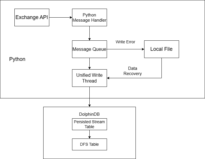
The collectionTime field in stream tables represents the local timestamp when real-time data is collected and can be used to analyze subscription latency.
2.3.2 Core Components
- _framework.py: General framework for data ingestion.
- xxxBaseConfig: Base configuration class defining common settings such as DolphinDB connection, proxy configuration, real-time queues, and cache files. It also provides methods for workflow startup, timeout monitoring, etc.
- IOThread: A common class that centrally manages the single write
path for MTW writing, local persistence, and data backfill,
executing serially to avoid disorder. It has following three states:
- live: DolphinDB is healthy; data is taken from the real-time queue and written via MTW.
- offline: DolphinDB is unavailable; real-time queue data is persisted locally as much as possible, then probed from the first local record after a cooldown period.
- replay: Only local cache data is written to MTW; the real-time queue is not consumed. After the local cache is cleared, the system switches back to the live state.
- <targetData>.py: Real-time data ingestion script.
- get_create_table_script: Table creation script defining the schema of stream tables and DFS tables. The script is run when rebuilding the writer to prevent stream table invalidation caused by server shutdowns.
- create_message_handler: Core handler that processes each subscribed message, parses fields, and converts them into the write format before pushing them into the queue for the writer thread. For OHLC data, only closed bars are processed.
2.3.3 State Transition Details
live state (normal operation)
Real-time data is fetched from the queue and written directly to DolphinDB via MTW, with write results monitored.
State transition condition
MTW write fails: live → offline
if self.mode == 'live':
    try:
        row = realtime_q.get(timeout=LIVE_GET_TIMEOUT)
        self._insert_one(row)  # Call MTW for writing
    except Exception as e:
        # Processing sequence for write failure
        save_unwritten_to_local()          # 1. Save MTW's internal cache
        self._append_rows_to_local([row])  # 2. Save rows failed to be written
        self._save_queue_to_local()        # 3. Save rows in the queue
        writer = None          # Mark MTW as invalid
        self.mode = 'offline'  # Switch to offline mode
        self.next_probe_ts = time.time() + PROBE_COOLDOWN_SECS # Set the time for next probing
offline state (local cache mode)
To prevent data loss, the system automatically caches data locally during DolphinDB failures. After the cooldown period, it probes for recovery and automatically backfills cached data once the system is recovered.
State transition condition
Probing succeeds and the database connection is recovered: offline → replay
elif self.mode == 'offline':
    now = time.time()
    if now < self.next_probe_ts:
        # Within cooldown period: only persist data locally
        self._save_queue_to_local(max_n=50000)  # Batch persistence to avoid blocking
        time.sleep(0.1)
        continue
    # Cooldown period ended: attempt to probe liveness
Probe mechanism: The system attempts a test write by reading and writing the first line of the local cache file. Success indicates that DolphinDB has recovered.
def _probe_from_local_first_line(self) -> bool:
    # 1. Ensure an available MTW; rebuild it if missing
    if writer is None and not build_mtw():
        return False
    # 2. Read and test the first line from the local file
    with file_lock:
        with open(self.path, "r", encoding="utf-8") as f:
            line = f.readline()
            if not line or not line.endswith("\n"):
                return False
            try:
                row = json.loads(line)
                self._insert_one(row)  # Attempt to write a single record
                return True            # Success indicates recovery; then switch to live state
            except Exception:
                writer = None
                return False
replay state (data backfill mode)
In this state, the real-time queue is not consumed to preserve historical data ordering. The system reads the local cache file in batches and writes data sequentially into the database. Large files are processed in batches to avoid memory overflow.
State transition conditions
- Local cache backfill completes successfully: replay → live
- Failure occurs during replay: replay → offline
def _replay_all_local(self) -> bool:
        global writer
        total = 0
        try:
            with file_lock:
                src = open(self.path, "r", encoding="utf-8", newline="\n")
                while True:
                    # Read in batches to avoid memory overflow
                    batch_lines = read_n_lines(READ_BATCH_SIZE)
                    if empty(batch_lines):
                        break
                    try:
                        # Batch write to the database
                        for line in batch_lines:
                            row = json.loads(line)
                            insert_one(row)
                        total += len(batch_lines)
                    except Exception as e:
                        # Roll back unwritten data and remaining records to local storage
                        return False
            # All records written successfully, clear the local file
            src.close()
            with file_lock, open(self.path, "w", encoding="utf-8"):
                pass
            print(f"[{time.strftime('%H:%M:%S')}] Backfill completed, {total} rows written, cache cleared")
            return True
        except Exception as e:
            print(f"[{time.strftime('%H:%M:%S')}] Backfill failed: {e} (cache retained, will retry)")
            writer = None
            return False
2.3.4 Variables and Usage Instructions
Before running, ensure that the target database and tables exist in the DolphinDB server. Modify the following variables according to your requirements and execute the Python script. The full script is provided in the Appendix.
| Variable | Location | Description |
|---|---|---|
| DDB | config.py | DolphinDB connection settings: host, port, username, password |
| PROXY | config.py | Proxy address; does not apply to OKX real-time data |
| TIMEOUT | config.py | WebSocket timeout in seconds; default: 5s |
| PROBE_COOLDOWN_SECS | config.py | Probe interval; default: 30s |
| READ_BATCH_SIZE | config.py | Maximum number of lines read per batch during backfill; default: 20000 |
| LIVE_GET_TIMEOUT | config.py | Blocking wait time in seconds when fetching data from the real-time queue in live mode; default: 0.2s |
| RECONNECT_TIME | config.py | WebSocket reconnection wait time (effective for OKX real-time data) |
| OKX_WS_URL | config.py | WebSocket server address (effective for OKX real-time data) |
| dbName | Target data file (global config) | Target database name for subscription-based writes |
| tbName | Target data file (global config) | Target table name for subscription-based writes |
| streamtbName | Target data file (global config) | Stream table name |
| BUFFER_FILE | Target data file (global config) | Local cache file path |
| symbols | Target data file (global config) | Symbols to import (Binance format), e.g. ["btcusdt"] |
| inst_ids | Target data file (global config) | Symbols to import (OKX format), e.g. futures ["BTC-USDT-SWAP"], spot ["BTC-USDT"] |
| script | Function in target data file: get_create_table_script() | Table schema; For details, refer to Section 2.1. |
The following example describes how to ingest level 2 futures data using Binance_Future_KLine.py. You can modify the corresponding parameters to ingest other types of data.
- Create the required databases and tables for the target data types. We recommend that you do not change database or table names. For the full script, refer to createDatabase.dos provided in the Appendix.
- Create the required stream tables. To enable persistence, add the
following parameter to the node configuration
file:
persistenceDir=/home/DolphinDB/Data/Persistence - Install the required dependencies in the Python environment.
Example:
pip install dolphindb pip install binance-connector pip install binance-futures-connector pip install websockets pip install python-okx pip install okx - Modify config.py and the configuration class BinanceBaseConfig in
Binance_Future_KLine.py as needed.
Example:
// config.py -- modify DDB and PROXY as needed DDB={"HOST":'192.168.100.43',"PORT":8848,"USER":'admin',"PWD":'123456'} BINANCE_BASE_CONFIG={"PROXY":'http://127.0.0.1:7890/', "TIMEOUT":5, "PROBE_COOLDOWN_SECS":30, "READ_BATCH_SIZE":20000, "LIVE_GET_TIMEOUT":0.2 } //... // Binance_Future_KLine.py -- modify as needed class BinanceFutureKLineConfig(BinanceBaseConfig): """Binance minute-level data ingestion configuration""" tableName = "Cryptocurrency_minKLineST" BUFFER_FILE = "./Binance_fKLine_fail_buffer.jsonl" symbols = ["btcusdt","ethusdt","adausdt","algousdt", "bnbusdt","fetusdt","grtusdt","ltcusdt","xrpusdt"] - Create a WebSocket connection, subscribe to the target market data, and
keep the main thread
running.
// Subscription function must be configured
def start_client_and_subscribe(self):
    // Create WebSocket connection
    client = UMFuturesWebsocketClient(
        on_message=self.create_message_handler(),
        proxies={'http': self.proxy_address, 'https': self.proxy_address}
    )
    // Subscribe to target symbols
    for s in self.symbols:
            client.kline(symbol=s,interval="1m")
            time.sleep(0.2)
    return client
# Usage
if __name__ == "__main__":
    config = BinanceFutureKLineConfig()
    client = config.start_all()
    # Keep main thread alive
    try:
        while True:
            time.sleep(1)
    except KeyboardInterrupt:
        config.quick_exit()
To ingest real-time OHLC data at different frequencies, modify the subscription parameters (interval for Binance, channel for OKX ). For example, modify line 10 in the above code. Supported real-time OHLC frequencies are consistent with historical OHLC frequencies (see Section 2.2). For OKX, the real-time OHLC frequency requires the channel prefix, such as 'candle1m' and 'candle3m'; other frequencies follow the same pattern.
2.4 Monitoring and Daily Scheduled Backfill
Due to the complexity and uncertainty of cryptocurrency exchange networks, exception handling and monitoring are critical. Therefore, scheduled jobs are configured in DolphinDB for data integrity monitoring and daily batch processing, with alerts sent via communication channels such as WeCom, reducing the difficulty of data maintenance in quantitative trading systems.
2.4.1 Real-Time Data Monitoring
Core functions
- Stream table health checks: Monitor subscription status of stream tables (e.g., level 2 data, trade details, OHLC data) to prevent ingestion interruptions.
- Real-time data checks: Monitor whether new data arrives in each table within 30 minutes to detect issues in data sources.
- Alerting: Send real-time alerts via WeCom bots to ensure timely response.
2.4.2 Daily Data Processing
Core functions
- Data integrity checks: Verify the completeness of minute-level OHLC data for the previous trading day (e.g., number of symbols × 1440 minutes × 2 markets).
- Automatic backfill: If data is missing, batch-fetch data via RESTful APIs for both futures and spot markets.
- Batch factor computation: Compute MyTT technical metrics, Alpha factors, etc., based on complete data that has been cleansed.
- Retry policy: Retry up to 10 times to mitigate transient network issues; if still failing after retries, send alerts via WeCom bots.
2.4.3 Usage Instructions
This section describes how to configure the system based on actual needs. For the full scripts, refer to checkData.dos and getCleanKLineAfterDay.dos provided in the Appendix.
- Determine the WeCom group to receive alerts and create a bot to obtain the Webhook URL.
- Update the webhook variable in the scripts with the actual bot URL.
- Verify that the monitored/processed database and table names match the actual environment.
- Process daily data (getCleanKLineAfterDay.dos):
- Modify codes in
getBinanceCleanData(), as well as future_inst_ids and spot_inst_ids ingetOKXCleanData()based on selected assets. - To add more factors, update factor definitions in
outputNamesMap()and verify the target tables for factor storage.
- Modify codes in
- Use
scheduleJobto add scheduled tasks and adjust execution times as needed.
2.5 Funding Rate Data Ingestion
Funding rates are a key metric of perpetual futures market sentiment and price deviation. Their sign and magnitude directly reflect long-short balance, providing important quantitative signals for trend analysis. Based on the characteristics of funding rate data, scripts are provided to batch-import historical data and to periodically fetch the latest data via scheduled jobs in DolphinDB.
Historical Data
Both Binance and OKX provide historical funding rate data; however, OKX only provides data of the most recent three months. Below, we use Binance's historical funding rate data as an example. The full script is provided in the Appendix.
getBinanceFundingRate: Fetches data from the exchange and parses it into the database.def getBinanceFundingRate(param,proxy_address,dbName,tbName){ //... config[`proxy] = proxy_address response = httpClient::httpGet(baseUrl,param,10000,,config) result = parseExpr(response.text).eval() tb = each(def(mutable d){ d["symbol"] = string(d.symbol) //... return d },result).reorderColumns!(`symbol`symbolSource`fundingTime`fundingRate`markPrice) loadTable(dbName,tbName).tableInsert(tb) }getFundingRate: Retrieves historical data for specified symbols and time ranges, with reconnection on failure.def getFundingRate(codes,startDate,endDate,proxy_address,dbName,tbName){ //... for(code in codes){ do{ param = dict(STRING, ANY) param["symbol"] = code param["startTime"] = startTimeUTC param["endTime"] = endTimeUTC param["limit"] = 1000 // Import with retry on failure getBinanceFundingRate(param,proxy_address,dbName,tbName) cursor += long(8)*3600*1000*1000 sleep(200) }while(cursor < endTimeUTC) } }
You only need to set the cryptocurrency list, start time, and target database/table names.
codes = ["btcusdt","ethusdt","adausdt"].upper()
proxy_address = "http://127.0.0.1:7890"
dbName, tbName= ["dfs://CryptocurrencyDay",`fundingRate]
getFundingRate(codes,2023.01.01,2025.10.05,proxy_address,dbName,tbName)
Real-time data
Since funding rates are updated every 8 hours, scheduled jobs are used to fetch them. Binance is used as an example below. The full script is provided in the Appendix.
getBinanceFundingRate: Calls the RESTful API to fetch funding rates, formats them into a vector usingparseExprandtranspose, and writes data to the target partitioned table.def getBinanceFundingRate(param,proxy_address,dbName,tbName){ //... config[`proxy] = proxy_address response = httpClient::httpGet(baseUrl,param,10000,,config) //... for(r in result){ r = select string(symbol),"Binance-Futures", timestamp(long(fundingTime)+8*3600*1000), double(fundingRate), double(markPrice) from r.transpose() loadTable(dbName,tbName).tableInsert(r) } }job_getFundingRate: Iterates over specified symbols and constructs the UTC start time. Requests are spaced by 200 ms to avoid rate limits. Modify the symbol list (codes) as needed (line 2). Alerts are sent on failure.def job_getFundingRate(webhook,proxy_address,dbName,tbName){ codes = ["btcusdt","ethusdt"].upper() // Use the timestamp from 2 minutes ago as the start time; schedule the job at :01 startTimeUTC = convertTZ(now()-2*60*1000, "Asia/Shanghai", "UTC") ts = long(timestamp(startTimeUTC)) for(code in codes){ param = dict(STRING, ANY) param["symbol"] = code param["startTime"] = ts getBinanceFundingRate(param) sleep(200) } if(errCnt == codes.size()){ msg = "Failed to fetch Binance fundingRate" sendWeChatMsg(msg,webhook) }
Configure scheduled jobs to fetch updated funding rates:
times = [08:01m, 16:01m, 00:01m]
proxy_address = 'http://127.0.0.1:7890'
dbName, tbName= ["dfs://CryptocurrencyDay",`fundingRate]
scheduleJob("fundingRateFetcher", "Fetch fundingRate",job_getFundingRate{proxy_address,dbName,tbName},times,
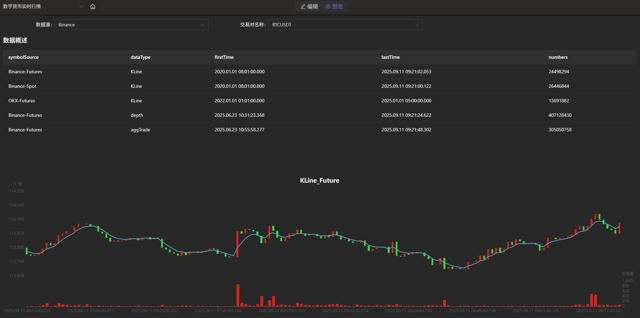
2025.06.17, 2035.12.31,"D")2.6 Market Data Visualization
After real-time market data ingestion, you can view live data in the DolphinDB data dashboard by importing the provided panel files. Dashboards support custom refresh intervals (e.g., 1 s). An example dashboard is shown below.
3. Unified Stream and Batch Processing for Factor Development
In quantitative trading, factor discovery is a critical step. Traditional approaches can be divided into manual discovery and algorithm-based discovery. Manual discovery relies heavily on researchers’ expertise and market insight, but it is inefficient, labor-intensive, and constrained by individual cognitive limits, making it difficult to fully capture the complex characteristics of the market. Algorithm-based discovery, on the other hand, leverages techniques such as machine learning to reduce manual costs. In particular, deep learning and neural networks, with their strong nonlinear fitting capabilities, can effectively capture complex nonlinear relationships among price-volume data, market sentiment, and macro or geopolitical factors in the cryptocurrency market, thereby generating factors that better reflect market fundamentals. Although deep learning models carry the risk of overfitting, this risk can be effectively controlled through proper model design, parameter tuning, and regularization, making them highly valuable for factor mining in cryptocurrency markets.
Training machine learning models for factor generation requires fast access to and processing of massive volumes of historical data. Traditional databases often suffer from low storage efficiency and slow query performance under such data scales. DolphinDB offers multiple advantages in quantitative factor discovery, significantly improving overall efficiency while aligning with practical requirements. Its built-in library of over 2,000 functions covering multiple domains and use cases provides fast and accurate data support for factor discovery, enabling machine learning models to be trained and optimized based on the latest market dynamics. In addition, DolphinDB’s streaming-batch framework allows you to efficiently perform batch factor computation while also supporting low-latency streaming computation, which can be applied in real time to cryptocurrency backtesting and simulated trading, closely approximating live trading conditions.
Accordingly, this chapter focuses on three aspects:
- How to design an optimal storage scheme for minute-level factor data based on DolphinDB;
- How to implement batch and streaming factor computation using DolphinDB’s built-in modules and plugins;
- How machine learning models are applied in backtesting and simulation.
3.1 Minute-Level Factor Database and Table Design
Given the characteristics of minute-level factor data and practical usage scenarios, we recommend using the TSDB storage engine and adopting a narrow-table schema with time and factor columns as partition keys. This design supports continuous growth in the number of factors while ensuring high write and query performance. The specific database and table design is as follows; the full script is provided in the Appendix.
| Database Name | Storage Engine | Partition Scheme | Partition Columns | Sort Columns | Partition Size |
|---|---|---|---|---|---|
| CryptocurrencyFactor | TSDB | Monthly partition + VALUE partition by factor name | Time + factor name | Market + asset + time | About 115.36 MB per single factor for 100 assets |
If the estimated number of combinations of market and asset exceeds 1,000, it
is recommended to reduce the dimension of the sort columns during database
creation by adding the following parameter:
sortKeyMappingFunction=[hashBucket{,3},
                            hashBucket{,300}]
.
The column definitions of the minute-level factor table (factor_1m) are as follows.
| Column Name | Data Type | Description |
|---|---|---|
| datetime | TIMESTAMP | Time column |
| symbol | SYMBOL | Asset for factor computation |
| market | SYMBOL | Market, such as ‘Binance-Futures’, ‘Binance-Spot’, ‘OKX-Futures’, ‘OKX-Spot’ |
| factorname | SYMBOL | Factor name |
| factorvalue | DOUBLE | Factor value |
3.2 Factor Computation
Taking DolphinDB’s built-in 191 Alpha and WorldQuant 101 Alpha factor libraries as examples, these factors were originally designed for the stock market. Therefore, cross-sectional and financial-statement-based factors are not applicable to the cryptocurrency market, and time-series factors are not defined as state functions. In this tutorial, applicable time-series factors are converted into state functions and stored in the stateFactors.dos file. You can load this module via use or modify it to develop custom factors. The full script is stateFactors.dos provided in the Appendix.
Using the gtjaAlpha100 factor as an example, we demonstrate how to perform both batch and streaming computation for the same factor in DolphinDB. In stateFactors.dos, gtjaAlpha100 is defined as:
@state
def gtjaAlpha100(vol){
    return mstd(vol, 20)
}
Compared with its definition in gtja191Alpha.dos, the only difference is the addition of @state, which converts it from a regular function into a state function, enabling direct use in streaming computation.
3.2.1 Batch Factor Computation
Factors are computed based on minute-level OHLC data, so historical minute-level OHLC data must exist in the DolphinDB server.
Batch computation consists of three steps: retrieving historical data, generating factor computation expressions, and computing and writing results to the database. The full script is provided in the Appendix.
- Retrieve historical data from the
database.
// Use the factor module use stateFactors go all_data = select * from loadTable("dfs://CryptocurrencyKLine","minKLine") factor_value_tb = loadTable("dfs://CryptocurrencyFactor", "factor_1min") - Generate factor computation
expressions.
cols_dict = {
    "vol": "volume"
}
def dict_replace_str(s, str_dict){
    for (i in str_dict.keys()){
        result = regexReplace(s, i, str_dict[i])
    }
    return result
}
use_func_call = exec name.split("::")[1]+syntax from defs() where name ilike "%stateFactors%"
funcName = func_call[:regexFind(func_call, "[()]+")]
deal_func_call = dict_replace_str(func_call, cols_dict)
select_string = stringFormat(
    "select eventTime,symbol,symbolSource,\"%W\" as factorname,
     %W as factorvalue from all_data
     context by symbol,symbolSource csort eventTime",
    funcName, deal_func_call)
Here,
dict_replace_strandcols_dictare used to replace parameter names in function expressions. For example, the parameter vol corresponds to the column volume in the database, allowing you to compute factors without modifying original column names. - Loop through all factors and append results to the
database.
for (func_call in use_func_call){// func_call=use_func_call[0]
    funcName = func_call[:regexFind(func_call, "[()]+")]
    deal_func_call = dict_replace_str(func_call, cols_dict)
    select_string = stringFormat("select eventTime,symbol,symbolSource,\"%W\" as factorname, %W as factorvalue from all_data context by symbol,symbolSource csort eventTime", funcName, deal_func_call)
    result = select * from parseExpr(select_string).eval()
    factor_value_tb.append!(result)
}
3.2.2 Streaming Factor Computation
Factors are computed based on minute-level OHLC data, so a minute-level OHLC stream table must exist.
Streaming factor computation includes three steps: creating a factor stream table, building a narrow reactive state engine, and subscribing to upstream data streams. The full script is provided in the Appendix.
- Create a persistent stream table to store computed factor
data.
// Stream table used to store factor data
output_stream = "min_factor_stream"
// Output table definition and conversion function
try{dropStreamTable(output_stream)}catch(ex){}
temp = streamTable(1:0, ["datetime","symbol","market","factorname","factorvalue"],
        ["TIMESTAMP","SYMBOL","SYMBOL","SYMBOL","DOUBLE"])
enableTableShareAndCachePurge(temp, output_stream, 10000000)
def output_handler(msg, output_stream){
    if (count(msg) == 0){return}
    cols = msg.columnNames()[2 0 1 3 4]
    tb = objByName(output_stream)
    tb.append!(<select _$$cols from msg>.eval())
}
//Used as a placeholder for output table in the engine with no actual effect.
try{dropStreamTable("output_tmp")}catch(ex){}
share streamTable(1:0, ["symbol","market","datetime","factorname","factorvalue"],
        ["SYMBOL","SYMBOL","TIMESTAMP","SYMBOL","DOUBLE"]) as output_tmp
Before building the reactive state engine that returns a table in narrow format, the output table and output handler must be created. The above code defines
output_handlerand two stream tables (output_stream and output_tmp). Theoutput_handlerfunction will serve as the outputHandler parameter for the engine. After setting this parameter, the results will no longer be written to the output table, but instead, output_handler will process the results. Therefore, the actual result writing happens at line 12 of the code. output_tmp is used as a placeholder, and after the engine is created, this stream table can be deleted. - Build the narrow reactive state
engine.
// List of required factor function names
func_table = select * from defs() where name ilike "%stateFactors%"
factor_fuc_name = func_table["name"].split("::")[1]
// List of factor metric computation meta-code
factor = [<eventTime>]
factor_fuc_syntax = parseExpr(func_table["name"] + func_table["syntax"])
factor.appendTuple!(factor_fuc_syntax)
engine_name = "cryto_cal_min_factor_stream"
// Try to drop the existing stream engine, if any
try { dropStreamEngine(engine_name) } catch (ex) {}
// Create the narrow reactive state engine
engine = createNarrowReactiveStateEngine(
    name=engine_name,
    keyColumn=["symbol", "symbolSource"], // Grouping columns
    metrics=factor, // Factor computation meta-code
    metricNames=factor_fuc_name, // Factor name
    dummyTable=table(1:0, ["eventTime", "collectionTime", "symbolSource", "symbol", "open", "high", "low", "close", "vol", "numberOfTrades", "quoteVolume", "takerBuyBase", "takerBuyQuote", "volCcy"], ["TIMESTAMP", "TIMESTAMP", "SYMBOL", "SYMBOL", "DOUBLE", "DOUBLE", "DOUBLE", "DOUBLE", "DOUBLE", "INT", "DOUBLE", "DOUBLE", "DOUBLE", "DOUBLE"]),
    outputHandler=output_handler{, output_stream},
    outputTable=objByName("output_tmp"),
    msgAsTable=true
)
try { dropStreamTable("output_tmp") } catch (ex) {}
To add custom factors, you only need to append factor names and computation logic to
factor_fuc_nameandfactor. - Subscribe to upstream data streams.
For example, subscribe to Cryptocurrency_minKLineST, the minute-level OHLC stream table.
input_stream = 'Cryptocurrency_minKLineST'
try{unsubscribeTable(,input_stream, "cal_min_factors")}catch(ex){}
subscribeTable(,input_stream, "cal_min_factors", getPersistenceMeta(objByName(input_stream))["memoryOffset"], engine, msgAsTable=true, throttle=1, batchSize=10)
3.3 Model Training and Real-Time Signal Generation
After factor computation and storage, machine learning models are trained and applied to backtesting and simulation for generating trading signals. The workflow consists of four steps:
- factor data retrieval and preprocessing;
- factor model training in Python;
- factor model export;
- trading signal prediction within DolphinDB combined with the backtesting and simulation framework. The fourth step supports both historical and real-time signal generation. The overall workflow is illustrated in Figure 3-1.

3.3.1 Data Retrieval and Preprocessing
Historically computed factor data is stored in dfs://CryptocurrencyFactor,
currently containing only 1-minute factors, with more frequencies to be
added in the future. To simplify factor data retrieval and standardization
in a Python client via the DolphinDB API, preprocessing is encapsulated in
the Python class FactorDataloader. All preprocessing is
executed on the DolphinDB server, and the Python client only receives the
processed data.
FactorDataloader provides preprocessing support for LSTM,
XGBoost, and Transformer models. Example:
from DataPre import FactorDataloader
ddb_connect = ddb.session("ip", port)
t = FactorDataloader(
    db_connect=ddb_connect,
    symbol="BTCUSDT",
    start_date="2024.03.01",
    end_date="2024.03.02",
    factor_name=["gtjaAlpha2"],
    market="Binance-Futures",
)
train_loader, test_loader = t.get_LSTM_dataloader(10, 0.2, 32)
train_loader, test_loader = t.get_xgboost_data(0.2)
train_loader, test_loader = t.get_transformer_data(1440, 0.2, 32)
3.3.2 Python Model Training
The DolphinDB’s GpuLibTorch plugin allows you to load and run the TorchScript model exported from Python, combining DolphinDB’s data processing capabilities with PyTorch’s deep learning functionality. You can run the following functions to install and load the GpuLibTorch plugin.
login("admin", "123456")
listRemotePlugins()
installPlugin("GpuLibTorch")
loadPlugin("GpuLibTorch")
The plugin does not support training models within DolphinDB, so training must be performed in a Python environment. A generic training and evaluation framework for three-class classification tasks is implemented in Models.py, supporting LSTM and Transformer models. The related functions are as follows:
# Functions
evaluate_classify_model(model, test_loader, device=torch.device("cuda" if torch.cuda.is_available() else "cpu"))
train_model(
    model,
    criterion,
    optimizer,
    num_epochs: int,
    train_loader,
    test_loader,
    device=torch.device("cuda" if torch.cuda.is_available() else "cpu"),
    per_epoch_show: int = 20,
)
# Usage
# Model training
criterion = nn.CrossEntropyLoss()
optimizer = optim.Adam(model.parameters(), lr=0.001, weight_decay=1e-5)
trained_model = train_model(
    model=model,
    criterion=criterion,
    optimizer=optimizer,
    num_epochs=100,
    train_loader=train_loader,
    test_loader=test_loader,
)
# Model evaluation
accuracy, preds, targets = evaluate_classify_model(trained_model, test_loader)
3.3.3 Model Export
After training in Python, the model needs to be exported as a model.pth file for prediction in DolphinDB. Models exported using torch.jit.trace may cause an error when loading in DolphinDB due to hidden layer tensors and input tensors not being on the same device. Therefore, we recommend that you use torch.jit.script to export the model file.
torch.jit.script(model).save("model.pth")3.3.4 Model Prediction and Backtesting/Simulation
Historical Computation Method
After obtaining the model, predictions can be made on upstream factor data using the GpuLibtorch plugin to generate trading signals for backtesting. This method requires pre-computed future signals and is suitable for backtesting only. For real-time simulation, the real-time computation method discussed later should be used.
table_name = "factor_predict_result"
try{
    undef(table_name, SHARED)
    print(table_name+" exists, stream table cleared")
} catch(ex) {
    print(table_name+" does not exist, environment cleaned")
}
share(table(100000: 0, `datetime`signal, [TIMESTAMP, INT]), table_name)
model = GpuLibTorch::load(model_file)
predict_result = GpuLibTorch::predict(model, data_input)
The above code creates a stream table named factor_predict_result to store the pre-computed signals for easy retrieval during backtesting. As shown in lines 9-10, you can load the trained model using GpuLibTorch and input pre-processed data (data_input) to get the model output (predict_result). The results are then inserted into the factor_predict_result stream table. The preprocessing of data_input is detailed in the DataPre.py script provided in the Appendix.
After obtaining the trading signal stream table factor_predict_result, it can be used in the event callback function for backtesting. The following example generates trading signals for BTCUSDT from 2025.03.01 to 2025.05.01 using an LSTM model, as shown in line 3. The callback function performs buy and sell operations based on the signal, as shown in lines 11 and 17. The full script is in the Appendix.
def onBar(mutable context, msg, indicator){
	//...
    singal_t = objByName("factor_predict_result")
    for(isymbol in msg.keys()){
        source = msg[isymbol]["symbolSource"]
        lastPrice = msg[isymbol]["close"]
        tdt = msg[isymbol]["tradeTime"]
        signal = exec signal from singal_t where datetime=tdt
        signal = signal[0]
        if (signal==int(NULL)){break}
        if (signal==0){
            // Sell
            qty = Backtest::getPosition(context["engine"], isymbol, "futures").longPosition
            if (qty > 0){
                Backtest::submitOrder(context["engine"], (isymbol, source, context["tradeTime"], 0, lastPrice, 0, 1000000, qty, 3, 0, 0, context["tradeTime"].temporalAdd(1m)), "sell", 0, "futures")
            }
        } else if (signal==2){
            // Buy
            Backtest::submitOrder(context["engine"], (isymbol, source, context["tradeTime"], 5, lastPrice, 0, 1000000, 0.001, 1, 0, 0, context["tradeTime"].temporalAdd(1m)), "buy", 0, "futures")
        }
    }
}
After the backtest is completed, the daily realized profit and loss curve can be plotted as shown in Figure 3-2:
result = select * from day where accountType="futures"
plot((double(result["realizedPnl"])), result["tradeDate"])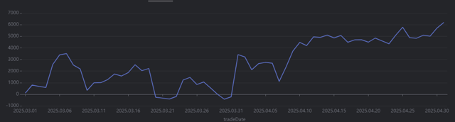
Real-time computation method
In addition to pre-computing trading signals for backtesting based on historical data, you can also simulate real-time trading by computing real-time factors and generating trading signals using a pre-trained model. This method is suitable for both historical market backtesting and simulated trading.
Below is the core code for a minute-level backtest demo that uses the gtjaAlpha94 and gtjaAlpha50 alpha factors for prediction. Since the factor computation functions in the built-in factor library of DolphinDB are not state functions, you need to use the factor computation functions that have been converted to state functions in the stateFactors module (see the previous section for module description).
- Pre-load the required model using a shared
dictionary.
// Initialize the model through a shared dictionary
model_dir = "/home/customer/model_config/test_LSTM.pth"
model = GpuLibTorch::load(model_dir)
GpuLibTorch::setDevice(model, "CUDA")
try{undef("test_ml_model", SHARED)}catch(ex){}
test_ml_model = syncDict(STRING, ANY, "test_ml_model")
go;
test_ml_model["model"] = model
This avoids reloading the model during subsequent computation. After loading the model, the GpuLibTorch::setDevice function must be called to specify the computing device for prediction. Otherwise, the default CPU will be used.
- Subscribe to signals in the
initializefunction to compute metrics.def gen_signal(factor1, factor2){ model = objByName("test_ml_model")["model"] data_input = matrix(zscore(factor1).nullFill!(0), zscore(factor2)).nullFill!(0).float() data_input = tensor(array(ANY).append!(data_input)) x = GpuLibTorch::predict(model, data_input)[0] signal = imax(1/(1+exp(x*-1))) return signal } def initialize(mutable context){ print("initialize load model") // Metric subscription indicator_dict = dict(STRING, ANY) indicator_dict["signal"] = <moving(gen_signal, (gtjaAlpha94(close.double(), volume.double()), gtjaAlpha50(high.double(), low.double())), 20)> Backtest::subscribeIndicator(context["engine"], "kline", indicator_dict, "futures") }By defining the meta-code in the initialize function, the backtesting engine can compute factor data in real time during backtesting and simulation. The corresponding model can be called in the signal computation function to generate signals. The event callback functions then obtain the trading signals through the indicator parameter. Here’s a usage example for the onBar callback function:
def onBar(mutable context, msg, indicator){
    //...
    one_msg = msg[isymbol]
    one_indicator = indicator[isymbol]
    signal = one_indicator["signal"]
    tdt = one_msg["tradeTime"]
    if (signal == int(NULL)){continue}
    if (signal == 0){
        // Sell
        qty = Backtest::getPosition(context["engine"], isymbol, "futures").longPosition
        if (qty > 0){
            Backtest::submitOrder(context["engine"], (isymbol, source, context["tradeTime"], 0, lastPrice, 0, 1000000, qty, 3, 0, 0, context["tradeTime"].temporalAdd(1m)), "sell", 0, "futures")
        }
    }else if (signal == 2){
        // Buy
        Backtest::submitOrder(context["engine"], (isymbol, source, context["tradeTime"], 5, lastPrice, 0, 1000000, 0.001, 1, 0, 0, context["tradeTime"].temporalAdd(1m)), "buy", 0, "futures")
    }
}
In the above onBar callback function, you can obtain the
real-time computed results of the signal generation function, which are
subscribed to in the initialize function, through the indicator
parameter, and then open or close positions based on the corresponding
signals. The full script is provided in the Appendix.
4. Strategy Backtesting and Simulated Trading
Before deploying a quantitative strategy to live trading, extensive backtesting and simulated trading are required to validate its effectiveness and feasibility. Mid- to high-frequency strategy backtesting and simulation for cryptocurrency trading face two major challenges. First, massive data storage and processing, especially for high-frequency snapshot data, which places extremely high demands on framework-level data processing and computational performance. Second, complex matching logic, where order execution must consider order price, traded volume, and market volatility, rather than simply using the latest price.
Leveraging its high-performance distributed architecture and low-latency streaming engine, DolphinDB integrates a backtesting engine with an order matching simulator to deliver an end-to-end backtesting and simulated trading solution. This solution supports market data replay and processing, strategy development and code management, result visualization, and strategy permission management. It supports both snapshot and minute-level cryptocurrency data, enabling individuals and quantitative teams to efficiently develop strategies with low code volume and a low learning curve. In addition to native DLang, strategies can also be written in Python and C++, offering high performance, low cost, and strong extensibility.
4.1 Cryptocurrency Backtesting Engine
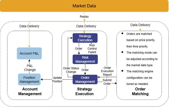
In DolphinDB, backtesting consists of four components: user-defined strategy functions, strategy configuration and creation, market data replay, and execution of the backtesting engine to obtain results. The cryptocurrency backtesting engine is provided as a plugin, and its logical architecture is shown in Figure 4-1. The main workflow includes:
- The engine replays market data streams in chronological order and dispatches them to the order matching simulator and market data callback functions.
- Market data callback functions process strategy logic and submit orders.
- The engine performs risk control management.
- Orders that pass risk control are sent to the order matching simulator for execution.
- The engine tracks positions and funds in real time, and returns strategy returns and trade details after backtesting completes.
The backtesting engine supports both snapshot and minute-level cryptocurrency data, and allows a single engine to manage multiple spot and futures accounts as well as different contract types. Cryptocurrency methods support specifying account operations via the accountType parameter.
When using DolphinDB for cryptocurrency strategy backtesting, the market data passed into the engine must strictly conform to the required data schema, often requiring substantial data cleansing and transformation. However, since strategy researchers prioritize designing and optimizing strategy logic, i.e., writing market callback functions, this solution streamlines the entire workflow. It not only provides raw exchange data, but also delivers processed and replay-ready snapshot and minute-level market data. Therefore, you can focus only on custom strategy functions and strategy configuration to quickly complete backtesting.
4.2 Strategy Development and Code Management
Market data access, backtest execution functions, trade simulation functions, and
code management for cryptocurrency backtesting are encapsulated in the
CryptocurrencySolution module. Based on the cryptocurrency
data environment built in Chapter 2, you can directly use this module to perform strategy
backtesting. The sub-modules are described below:
| Sub-module | Catagory | Description |
|---|---|---|
CryptocurrencySolution::utils |
Common functions | Includes common functions such as engine deletion and management, funding rate retrieval, base information tables, OHLC data downsampling, backtest and simulation strategy retrieval, strategy log retrieval, and database/stream table status checks. |
CryptocurrencySolution::setting |
Unified settings | Includes unified strategy configuration, GitLab address configuration, module lists, and database/table metadata. |
CryptocurrencySolution::runBacktest |
Backtesting | Includes market data retrieval and processing functions, and backtest execution functions. |
CryptocurrencySolution::simulatedTrading |
Simulation | Includes market data retrieval and processing functions, and simulation start/stop function. |
CryptocurrencySolution::manageScripts |
Code storage | Includes strategy upload, retrieval, and deletion functions, backtest result storage and retrieval functions, and backtest/simulation code submission and storage function. |
First, obtain the home directory using getHomeDir(), place the attached module folder in the corresponding path, and load it using use:
use CryptocurrencySolution::manageScripts
go
To meet strategy storage and management requirements, this solution integrates with GitLab. When submitting a strategy for backtesting or simulation, the system automatically uploads the strategy code to a specified Git repository, enabling unified management, version tracking, and rapid retrieval. For details, see Section 4.4.
If strategy code storage is not required, you can use the following modules for backtesting or simulation only:
// Backtesting
use CryptocurrencySolution::runBacktest
go
// Simulation
use CryptocurrencySolution::simulatedTrading
go
4.2.1 Writing Cryptocurrency Strategies
In this section, we introduce how to write cryptocurrency strategies. More detailed examples are provided in Chapter 5.
User-defined event callback functions
The backtesting engine adopts an event-driven mechanism and provides the following event functions. You can customize callbacks for strategy initialization, daily pre-market processing, snapshot and OHLC market data, and order and trade reports.
| Event Function | Description |
|---|---|
initialize(mutable context) |
Strategy initialization function: triggered once. The parameter context represents the logical context. In this function, you can use context to initialize global variables or subscribe to metric computation. |
beforeTrading(mutable context) |
Callback executed during the daily session rollover; triggered once when the trading day switches. |
onSnapshot(mutable context, msg) |
Snapshot market data callback. |
onBar(mutable context, msg) |
Low- to mid-frequency market data callback. |
onOrder(mutable context, orders) |
Order report callback, triggered whenever an order’s status changes. |
onTrade(mutable context, trades) |
Trade execution callback, triggered when a trade occurs. |
finalize(mutable context) |
Triggered once before strategy termination. |
- If GitLab-based strategy code management is required, the strategy must be declared using module, and the module name must match strategyName.
- Required modules used in callbacks must be listed in getUsedModuleName() in CryptocurrencySolution::setting. Otherwise, strategy code will fail to be uploaded.
module testMinStrategy   //Declare the strategy module when enabling code management
def initialize(mutable context){
}
def beforeTrading(mutable context){
}
def onBar(mutable context,msg, indicator){
}
def onSnapshot( mutable context,msg, indicator){
}
def onOrder( mutable context,orders){
}
def onTrade(mutable context,trades){
}
def finalize (mutable context){
}
strategyName = "testMinStrategy"
4.2.2 Cryptocurrency Strategy Configuration
The userConfig strategy configuration must include the strategy type,
backtest start and end dates, market data type, initial capital, and the
cryptocurrency asset to be backtested. The
CryptocurrencySolution::setting module provides default
strategy configuration, which can be obtained using the following
function:
startDate = 2025.08.24
endDate = 2025.08.25
dataType = 3 // Minute-level market data; set to 1 for snapshot data
userConfig = CryptocurrencySolution::setting::getUnifiedConfig(startDate, endDate, dataType)
An example of the userConfig is shown below:
sym = ["BTCUSDT"]
userConfig = dict(STRING,ANY)
userConfig["startDate"] = 2025.08.24
userConfig["endDate"] = 2025.08.25
userConfig["strategyGroup"] = "cryptocurrency"
cash = dict(STRING,DOUBLE)
cash["spot"] = 1000000.
cash["futures"] = 1000000.
cash["option"] = 1000000.
userConfig["cash"] = cash
userConfig["dataType"] = 3    // 1: snapshot; 3: minute-level
userConfig["Universe"] = sym  // Symbol for backtesting (required)
p = dict(STRING,ANY)
p["Universe"] = userConfig["Universe"] + "_futures"
p["log"] = table(10000:0,[`tradeDate,`time,`info],[DATE,TIMESTAMP,STRING]) // log table for debugging
userConfig["context"] = p    // Pass the asset universe
To backtest historical market data, you can customize the start and end dates in userConfig. This module automatically loads the default strategy configuration and allows user-provided userConfig values to override the defaults. By default, Binance data is used, and the backtest period is the most recent 10 days.
userConfig = dict(STRING,ANY)
userConfig["startDate"] = 2025.08.24
userConfig["endDate"] = 2025.08.25
// Example: backtest an asset (used to define the asset universe)
p = dict(STRING,ANY)
p["Universe"] = ["XRPUSDT_futures"]
userConfig["context"] = p
strategyType = 0
engine, straname_ =
    CryptocurrencySolution::manageScripts::runCryptoAndUploadToGit(
        strategyName, eventCallbacks, strategyType, userConfig
    )
To downsample OHLC data, you can use the built-in downsampling function and specify the barMinutes parameter:
strategyType = 0
engine, straname_ =
    CryptocurrencySolution::manageScripts::runCryptoAndUploadToGit(
        strategyName, eventCallbacks, strategyType, , barMinutes = 1
    )
To use market data from the OKX exchange, specify exchange =
"OKX". Otherwise, it defaults to "Binance":
engine, straname_ =
    CryptocurrencySolution::manageScripts::runCryptoAndUploadToGit(
        strategyName, eventCallbacks, strategyType, exchange = "OKX"
    )
4.2.3 Strategy Backtest Execution and Result Retrieval
After setting the strategyName, eventCallbacks, and
strategyType parameters, call
runCryptoAndUploadToGit to execute the backtest.
strategyName = "testMinStrategy"
eventCallbacks = {
    "initialize": initialize,
    "beforeTrading": beforeTrading,
    "onBar": onBar,
    "onOrder": onOrder,
    "onTrade": onTrade,
    "finalize": finalize
}
// Execute backtest and upload strategy files to GitLab
strategyType = 0
engine, straname_ =
    CryptocurrencySolution::manageScripts::runCryptoAndUploadToGit(
        strategyName, eventCallbacks, strategyType
)- During backtest execution, the strategy files are automatically uploaded to the specified GitLab repository, and the corresponding commit ID is stored in the gitstrategy table of the database dfs://CryptocurrencyStrategy.
- If strategy code management is not required, you can use
runCryptoBacktestfrom theCryptocurrencySolution::runBacktestmodule. This function automatically loads default strategy configuration and allows you to override it with a custom userConfig. By default, it performs backtesting on Binance data for the most recent 10 days.
// userConfig = dict(STRING,ANY)
// userConfig["startDate"] = 2025.11.10
// userConfig["endDate"] = 2025.11.20
engine, straname_ =
    CryptocurrencySolution::runBacktest::runCryptoBacktest(
        strategyName, eventCallbacks, userConfig
    )
Retrieve backtest results
After the backtest completes, you can retrieve daily positions, daily equity, return summary, trade details, and strategy configurations using the following methods.
// Trade details
tradeDetails = Backtest::getTradeDetails(engine, "futures")
// Unfilled orders
tradeDetails[tradeDetails.orderStatus == -3]
// Current open (unfilled) orders
Backtest::getOpenOrders(engine, "futures")
// Daily positions
Backtest::getDailyPosition(engine, "futures")
// Overall backtest summary
Backtest::getReturnSummary(engine)- After the backtest completes, the strategy return summary and configuration are stored in dfs://CryptocurrencyStrategy/backtestStrategy for comparative analysis.
- Visualization of backtest results is described in Section 4.3.
4.2.4 Submitting Simulated Trading
After real-time market data is ingested into stream tables, set
strategyType = 1 to enable simulated trading. The
strategy name will automatically be suffixed with SimulatedTrading, and the
strategy code will be managed and stored.
You can use the overwrite parameter to control whether strategies with the same name are automatically deleted (defaults to false). By default, Binance data is used and simulation starts from the current day.
strategyType = 1
engine, straname_ =
    CryptocurrencySolution::manageScripts::runCryptoAndUploadToGit(
        strategyName, eventCallbacks, strategyType,
        userConfig = NULL, overwrite = false
    )
After simulation starts, trade details, real-time positions, and equity are written in real time to the corresponding simulation tables, for example:
- strategyName + "_tradeDetails"
- strategyName + "_position"
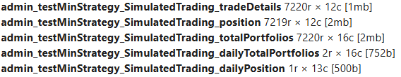
If strategy code management is not required, you can run simulated trading
using the submitCryptoSimulatedTrading function in the
CryptocurrencySolution::simulatedTrading module. This
function automatically loads the default strategy configuration and allows
you to override it with a custom userConfig. To run a simulation
based on an existing backtest strategy, use the
submitCryptoSimulatedTradingByStrategyName function,
which submits the backtest strategy (strategyName_) in
simulation mode.
// Directly submit simulated trading
engine, straname_ = submitCryptoSimulatedTrading(strategyName, eventCallbacks)
// Submit simulated trading based on an existing backtest strategy
engine, straname_ = submitCryptoSimulatedTradingByStrategyName(strategyName_, overwrite = false)4.2.5 Retrieving Strategy Logs
To simplify debugging, you can write logs inside strategy callback functions:
def beforeTrading(mutable context){
    // Write logs to the engine-maintained log table
    context.log.tableInsert(context["tradeDate"], now(), "beforeTrading")
}
Use getStrategyLog to retrieve strategy logs. If you define
a custom userConfig, you must manually add log settings.
CryptocurrencySolution::utils::getStrategyLog(straname_)Sample strategy logs:
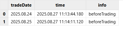
4.2.6 Deleting Strategies
To avoid excessive engine creation, each user is limited to a maximum of 5 strategy engines. Unneeded engines can be removed using dropMyBacktestEngine. For simulated strategies, the corresponding result tables are also deleted. You can only delete strategies created by yourself.
use CryptocurrencySolution::utils
straname_ = 'admin_testMinStrategy'
dropMyBacktestEngine(straname_)
4.2.7 Strategy Code Management
To meet requirements for strategy code storage and versioning, we integrate
backend modules with a GitLab repository. When a backtest or simulation is
submitted, the backend automatically uploads the strategy event callback
functions to a user-defined GitLab repository and records version
information in the corresponding database tables. All GitLab-related
strategy management functions are encapsulated in the
CryptocurrencySolution::manageScripts module.
First, you must create a GitLab account and obtain a GitLab Personal Access
Token for authentication. See Personal access tokens | GitLab
Docs for details. When using strategy code management, you can
either pass gitInfo or configure it globally in the
CryptocurrencySolution::setting module. Example:
gitInfo = dict(STRING,ANY)
gitInfo[`gitLabSite] = "https://dolphindb.net"   // GitLab URL
gitInfo[`repoId] = 620                          // Project ID
gitInfo[`repoBranch] = "main"                   // Branch name
gitInfo[`privateToken] = "zQx-BzyJrHxd_sbnEFNR"  // Access token
Below are the main functions provided by this module, including uploading, retrieving, and deleting strategies.
Upload strategy files
def uploadOrupdateToGit(
    strategyName, strategyType, eventCallbacks,
    gitInfo = NULL, commitMsg = NULL, timeout = 10000
)
Parameter description
| Parameter | Type/Form | Description | Required |
|---|---|---|---|
| strategyName | SYMBOL | Strategy name | Yes |
| strategyType | INT | Strategy type (0: backtest, 1: simulation) | Yes |
| eventCallbacks | DICT | Event callback functions | Yes |
| gitInfo | DICT | GitLab configuration; an example is displayed at the start of the section. | No |
| commitMsg | STRING | Commit mesaage | No |
| timeout | INT | Request timeout | No |
As described in Section 4.2, you can run backtests or simulations via
runCryptoAndUploadToGit, which automatically uploads
strategy code. Strategy versions (both new and updated) are recorded in
dfs://CryptocurrencyStrategy/gitstrategy. You can retrieve specific versions
using the stored commit IDs.
Retrieve strategy files
def getStrategyFromGit(
    strategyName, commitId = NULL, gitInfo = NULL, timeout = 10000
)
Parameter description
| Parameter | Type/Form | Description | Required |
|---|---|---|---|
| strategyName | SYMBOL | Strategy name | Yes |
| commitId | STRING | ID of the commit that uploads the strategy | No |
| gitInfo | DICT | GitLab configuration; an example is displayed at the start of the section. | No |
| timeout | INT | Request timeout | No |
By default, this function retrieves the latest version of the strategy. To fetch a specific version, specify commitId based on the records in dfs://CryptocurrencyStrategy/gitstrategy.
Delete strategy files
def deleteStrategyFromGit(
    strategyName, gitInfo = NULL, timeout = 10000
)
Parameter description
| Parameter | Type/Form | Description | Required |
|---|---|---|---|
| strategyName | SYMBOL | Strategy name | Yes |
| gitInfo | DICT | GitLab configuration | No |
| timeout | INT | Request timeout | No |
This function deletes the corresponding strategy file from GitLab. Use with caution. You can only delete strategies uploaded by yourself.
Submit backtests or simulations with code upload
def runCryptoAndUploadToGit(
    strategyName, eventCallbacks, strategyType, userConfig = NULL,
    barMinutes = 1, overwrite = false, gitInfo = NULL,
    commitMsg = NULL, timeout = 10000
)
Parameter description
| Parameter | Type/Form | Description | Required |
|---|---|---|---|
| strategyName | SYMBOL | Strategy name | Yes |
| eventCallbacks | DICT | Event callback functions | Yes |
| strategyType | INT | Strategy type (0: backtest, 1: simulation) | Yes |
| userConfig | DICT | Strategy configuration (Only start/end time can be modified; defaults are defined in setting) | No |
| exchange | STRING | Exchange providing the source data (default: "Binance"). | No |
| barMinutes | INT | Frequency in minutes, effective for OHLC data only. | No |
| overwrite | BOOL | Whether to delete existing simulation strategies with the same name (default: false). | No |
| gitInfo | DICT | GitLab configuration | No |
| commitMsg | STRING | Commit mesaage | No |
| timeout | INT | Request timeout | No |
This function wraps backtest/simulation submission and strategy code upload, using default strategy configuration. You only need to define strategyName, eventCallbacks, and strategyType to quickly deploy a cryptocurrency strategy. For details, see Section 4.2.3.
4.3 Strategy Result Visualization
To help you analyze backtesting and simulated trading results more intuitively, we provide separate dashboards for backtesting and simulation. These dashboards enable visual strategy management. You only need to import the dashboard files included in the Appendix—no additional configuration is required.
4.3.1 Backtesting Strategy Visualization
The backtesting dashboard displays all backtesting strategies and their results. It includes the following content:
- Strategy list
Shows the strategy names, engine status, error messages, and related information.

- Backtesting results
Select a strategy name and click Query to retrieve the backtesting results.
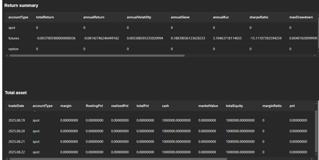
- Submit strategy for simulation
You can submit strategies that have been backtested for simulated trading. The simulation strategies will appear in the simulation dashboard.
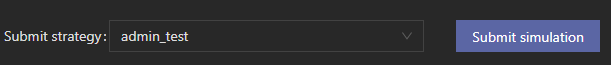
- Delete backtesting strategies
You can delete unneeded backtesting strategies.

4.3.2 Simulated Trading Strategy Visualization
The simulation dashboard displays all simulated trading strategies and their results. Its structure is the same as the backtesting dashboard. The page refreshes once per second to display real-time strategy results.
- Simulation strategy list
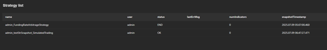
- Real-time trades and positions
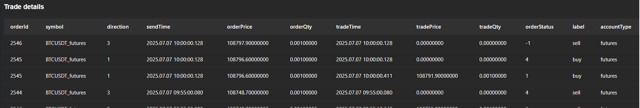
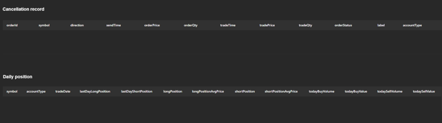
- Delete simulation strategies
You can delete unneeded simulation strategies.
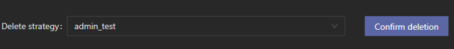
- Stop simulated trading
Simulation strategies that are no longer needed can be stopped. After stopping, the strategy will appear in the backtesting dashboard.

4.4 Strategy Permission Management
To support strategy isolation within quantitative teams, we implement user-level permission isolation for both backtesting and simulation strategies. Each user can only view the backtesting and simulation results they created, and strategy code is stored in user-defined GitLab repositories.
To use the cryptocurrency data environment for backtesting or simulation, contact the admin to create a user account with the required read permissions on the relevant databases and tables. Then, you can log in as the created account and import the dashboard files to view backtesting and simulation strategies. A permission granting script is shown below:
// Executed by admin
login("admin","DolphinDB123456")
// Create a new user
createUser("user1","123456",,false)
// Grant database and table permissions
grant(`user1, DB_READ, "dfs://CryptocurrencyDay")
grant(`user1, DB_INSERT,"dfs://CryptocurrencyStrategy")
grant(`user1, TABLE_READ, "P1-node1:Cryptocurrency_depthTradeMerge")
// Function view permissions
grant("user1", VIEW_EXEC, "CryptocurrencySolution::utils::getSimulatedTradingEngine")
grant("user1", VIEW_EXEC, "CryptocurrencySolution::utils::getAllBacktestEngine")
// Dashboard permissions
dashboard_grant_functionviews(`user1, NULL, false)
// Grant permissions to group member bk
grant(`bk, VIEW_EXEC, objs="CryptocurrencySolution::utils::getSimulatedTradingEngine")
grant(`bk, DB_INSERT, "dfs://CryptocurrencyStrategy")   // Permission on database storing backtesting results
grant(`bk, VIEW_OWNER) // Strategy storage requires function view permissionIf you want to share strategy backtesting results, use the dashboard sharing feature. Shared dashboards are view-only.
For centralized management, the following functions are restricted to the admin user:
- Unsubscribe all minute-level or snapshot stream
tables.
CryptocurrencySolution::utils::unsubscribeTableByAdmin(tbName)
- Retrieve return comparisons for all simulated
strategies.
CryptocurrencySolution::utils::getReturnComparision(startDate, endDate)
- Rebuild the database for strategy IDs and backtesting results. (Write
permissions must be re-granted to the specific user after
rebuilding.
CryptocurrencySolution::utils::createdatabase()
5. Live Trading
In a quantitative trading system, live trading is the final stage where strategies are put into real execution. Therefore, we integrated the trading and account APIs of Binance and OKX, and developed a live trading module based on DolphinDB’s httpClient plugin.
This module supports order placement, order cancellation, querying open orders, and retrieving trade details. It is consistent with the DolphinDB’s backtesting and simulation framework, allowing strategy backtesting, simulation, and live trading to share the same codebase. This significantly reduces the learning cost. Below is a description of the supported live trading functions. For details, see the Appendix.
| Module Function | Description | Notes |
|---|---|---|
submitOrder |
Places an order. | Returns order IDs (orderId and newClientOrderId). All order details and error information are stored in a stream table. |
cancelOrder |
Cancels an order. | No return value. All cancellation information is stored in the same stream table. |
getOpenOrders |
Gets open orders. | Returns information on unfilled orders. |
getTradeDetails |
Get trade details | Returns the latest 500 order records for a given asset. |
To record live trading information, the module maintains a persistent stream table, named by default as <username> + Cryptocurrency + '_BinanceTradeDetails' or<username> + Cryptocurrency + '_OKXTradeDetails'. This table stores real orders, network errors, exchange API errors, and other related information, making it easier for you to query orders and troubleshoot issues while avoiding frequent API calls that may be rejected. The detailed table schema is provided in the Appendix.
5.1 Prerequisites
Before live trading, you must obtain the API key and HMAC key for your personal or test account to ensure trading security.
Binance
- Register and log in to a Binance account.
- Go to API Management in the account settings to obtain the API key and HMAC key.
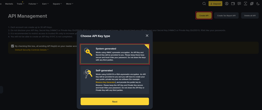
If you do not want to trade with a personal account for now, you can use the Binance Spot Test Network.
- Log in to your Binance account and sign in using a GitHub account.
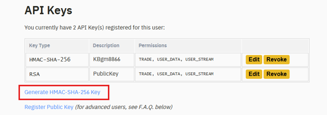
Figure 13. Figure 5-2: Obtain keys on the Binance test site - Click Generate HMAC-SHA-256 Key to generate the required keys.
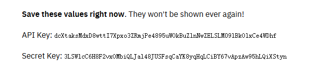
Figure 14. Figure 5-3: Generate keys on the Binance test site
OKX
- Register and log in to an OKX account.
- Go to the API section in the account settings and create an API
key.
Figure 15. Figure 5-4: Obtain API keys on OKX - Fill in the IP whitelist and passphrase, and select key permissions (read,
withdraw, trade) as needed.
Figure 16. Figure 5-5: Creating an API key on OKX Note:- If you do not have a static IP address, it is not recommended to set an IP whitelist, as IP changes may cause order failures.
- API keys without a bound IP address will be automatically deleted after 14 days of inactivity.
- After creation, click View to obtain the API key and secret. Please store them securely.
5.2 Implementation Steps
This section describes how to apply a simulated trading strategy to live trading. The full script is provided in the Appendix. For strategy development, see Section 4.2.1.
- Compile the OKX signature plugin (Linux). For compilation details,
see the plugin document.
- Download the DolphinDBPlugin project based on your server version, and place the source code (hex2Base64-main.zip) in the root directory.
- Run the following commands to generate .so and .txt files in the output folder.
- Place the output/hex2Base64-main folder in the server/plugins directory.
cd ../DolphinDBPlugin/hex2Base64-main export CMAKE_INSTALL_PREFIX="$(pwd)/output/$PluginName" # Default ABI1 export CXXFLAGS="-D_GLIBCXX_USE_CXX11_ABI=0" # Specify ABI0 via environment variable CXX=g++-8 CC=gcc-8 bash -x ./build.sh # Modify compiler version as needed - Place the
CryptocurrencySolutionmodule in the modules directory under the home directory (getHomeDir()), move files in CryptocurrencyTrading.zip to the CryptocurrencySolution directory, and modify the OKXTradingModule.dos file based on the plugin path.try{loadPlugin("/.../server/plugins/hex2Base64-main/PluginHex2Base64.txt")}catch(ex){print(ex)} go - Load the modules as
follows:
use CryptocurrencySolution::simulatedTrading use CryptocurrencySolution::CryptocurrencyTrading go - Retrieve and store asset precision
information.
tb = CryptocurrencySolution::CryptocurrencyTrading::getAssetPrecision() dbName = "dfs://CryptocurrencyDay" tbName = "precision" colNames = `symbol`symbolSource`contractType`tickSize`stepSize colTypes = [SYMBOL,STRING,STRING,DOUBLE,DOUBLE] if(!existsDatabase(dbName)){ db = database(dbName,RANGE,2010.01M+(0..20)*60) }else{ db=database(dbName)} if(!existsTable(dbName,tbName)){ createDimensionTable(db,table(1:0,colNames,colTypes),tbName) } loadTable(dbName,tbName).append!(tb) - Configure account credentials in
userConfig["context"].p = dict(STRING,ANY) // Key information – fill in with actual keys keyInfo = dict(STRING,ANY) keyInfo["apiKey"] = "" keyInfo["secretKey"] = "" // OKX requires an additional passphrase // keyInfo["passphrase"] = "123456" p["keyInfo"] = keyInfo userConfig["context"] = p - Example: placing orders in a minute-level strategy. Orders are placed in the
onBar callback. In the submitOrder function, isSim indicates whether the
order is placed in live trading or simulation mode, and it must match the
applied API
key.
Lines 8 and 12 show that the live order placement function is largely consistent with that of the backtesting plugin. Indef onBar(mutable context, msg, indicator){ endTime = timestamp() for(istock in msg.keys()){ source = msg[istock]["symbolSource"] buyPrice=msg[istock]["close"]+10 sellPrice =msg[istock]["close"]-10 if(context["number"]< 5){ submitOrder(context["keyInfo"],(istock,source,context["tradeTime"],5,buyPrice,0.0,0.0,0.01,1,0,1,endTime),"testOrders_buy", orderType=0, accountType ="futures",exchange = "Binance",paramDict=NULL,strategyName=context["strategyName"],isSim=true, proxy=NULL) context["number"] += 1 }else{ submitOrder(context["keyInfo"],(istock,source,context["tradeTime"],5,sellPrice,0.0,0.0,0.01,3,0,1,endTime),"testOrders_sell", orderType = 0, accountType = "futures",exchange = "Binance", paramDict = NULL,strategyName = context["strategyName"],isSim = true, proxy = NULL) con} def onOrder(mutable context,orders){} def onTrade(mutable context,trades){text["number"] -= 1 } } } def onOrder(mutable context,orders){} def onTrade(mutable context,trades){}Backtest::submitOrder, the first engine parameter must be replaced with the account credential information keyInfo. Cryptocurrency exchanges support more order parameters. Extensible parameters are passed via paramDict. For details, see New Order | Binance Open Platform and POST / Place Order – OKX API Documentation. - Submit the strategy using submitCryptoSimulatedTrading. Real-time market
data will enter the engine and trigger the callbacks to execute live
trading.
engine,straname_ = CryptocurrencySolution::simulatedTrading::submitCryptoSimulatedTrading(strategyName,
eventCallbacks, userConfig, overwrite = true)
If you need to store live trading strategy code, use the
CryptocurrencySolution::manageScripts module and add
keyInfo in the unified configuration function under
CryptocurrencySolution::setting, or pass keyInfo
via a custom userConfig. Other usage is the same as backtesting and
simulation. For details, see Chapter 4.
Live trading details can be obtained from the stream table (e.g., admin_testSubmitRealOrder_BinanceTradeDetails, shown in Figure 5-6). Successful order placements and cancellations are recorded in this table. If an order fails due to network issues or API errors, the error information is also stored, making it easy to review order status or diagnose failures.

You can retrieve open orders and trade details using the following functions:
openOrders_s = getOpenOrders(keyInfo,"BTCUSDT_spot")
openOrders_f = getOpenOrders(keyInfo,"BTCUSDT_futures", accountType="futures")
tradeDetails_s = getTradeDetails(keyInfo,"BTCUSDT_spot", accountType="spot")
tradeDetails_f = getTradeDetails(keyInfo,"BTCUSDT_futures", accountType="futures")
6. Real-Time Risk Control
Risk management is critical for investors, especially in the highly volatile cryptocurrency market. Based on DolphinDB, we implement a real-time portfolio risk management solution that integrates exchange account data. By periodically polling and calculating metrics such as portfolio net value, unrealized P&L, total value, and leverage ratio, the solution helps investors better understand and manage risk. The solution supports both Binance and OKX. The main module functions are as follows:
- Exchange data retrieval: Periodically retrieves real-time data such as wallet balances, futures positions, and market quotes from exchanges, and writes them into DolphinDB stream tables for subsequent computation.
- Real-time risk computation: Periodically computes risk metrics for spot and futures accounts using DolphinDB, and then combines both to derive overall portfolio risk metrics.
- Real-time data persistence: Persists account information and risk metrics to the DolphinDB database in real time for subsequent simulation and analysis.
6.1 Risk Metric Computation
This solution first computes risk metrics for spot and futures accounts separately, and then combines them to obtain overall portfolio risk metrics. The data involved includes spot and futures asset information, spot and futures price data, and futures position data. The formulas and variable names follow Binance’s definitions.
Spot account risk metrics
- Free value (freeValue): The sum of each asset’s free quantity multiplied by its corresponding market price (midPrice).
- Locked value (lockedValue): The sum of each asset’s locked quantity multiplied by its corresponding market price (midPrice).
- Spot total value (spotTotalValue): The sum of free value and locked value.
Futures account risk metrics
- Live unrealized P&L (liveUnrealizedProfit): The sum of potential profits across all futures positions based on the difference between the current market price and the break-even price.
- Futures net value (futuresNetValue): The sum of the total futures account value and unrealized profit.
- Total futures position value (principleAmt): The sum of each futures position multiplied by its corresponding market price (midPrice).
- Futures leverage ratio (futuresLeverageRatio): The total futures position value divided by the total futures account balance.
In the leverage computation, the discountRatio parameter is introduced as a conservative adjustment factor to prevent excessive leverage. In this solution, the discount ratio is set to 0.95.
Overall risk metrics
- Total value (totalValue): The sum of spot total value and futures net value.
- Total leverage ratio (totalLeverageRatio): The ratio of (spot free value plus the total futures position value) to the total account value.
6.2 Risk Model Construction
This section describes how to build the real-time risk model and configure real-time alerts. Binance is used as an example. The full script is provided in the Appendix.
Create data tables
In DolphinDB, create in-memory tables to store exchange data. Use
latestKeyedTable to create key-value in-memory tables for
account information (asset and position data) and price data, and share them
across all sessions on the current node using share. Key-value
in-memory tables make it easy to store the latest data and can be directly used
for risk metric computation. The following example shows how to create a spot
position table:
// Spot position
colNames = `asset`free`locked`updateTime
colTypes = [SYMBOL, DOUBLE, DOUBLE, TIMESTAMP]
share latestKeyedTable(`asset, `updateTime, 1000:0, colNames, colTypes) as spotBalanceKT
go
For risk metrics, use streamTable to create stream tables, and
enable enableTableShareAndPersistence to allow both sharing and
persistence.
// Risk metrics
colNames = `freeValue`lockedValue`spotTotalValue`baseCurrency`free`locked`balance`crossWalletBalance`crossUnPnl`availableBalance`maxWithdrawAmount`updateTime`principleAmt`liveUnrealizedProfit`unrealizedProfit`futuresNetValue`futuresLeverageRatio`totalValue`totalLeverageRatio
colTypes = [DOUBLE,DOUBLE,DOUBLE,STRING,DOUBLE,DOUBLE,
            DOUBLE,DOUBLE,DOUBLE,DOUBLE,DOUBLE,TIMESTAMP,DOUBLE,
            DOUBLE,DOUBLE,DOUBLE,DOUBLE,DOUBLE,DOUBLE]
enableTableShareAndPersistence(
    table=streamTable(10000:0, colNames, colTypes),
    tableName="portfolioRiskIndicatorST",
    cacheSize=100000,
    preCache=10000
)
go
Retrieve exchange data
Binance provides RESTful APIs for account information (assets and positions) and trading data. Using DolphinDB’s httpClient plugin, these data can be retrieved and written synchronously into DolphinDB tables.
- Account information: Retrieved via background jobs that poll every minute
and compute metrics. An example of fetching spot account information is
shown
below:
def getBinanceSpotAccount(keyInfo,proxy=NULL){
    apiKey = keyInfo["apiKey"]
    secretKey = keyInfo["secretKey"]
    baseUrl = 'https://testnet.binance.vision/api/v3/account'
    config = dict(STRING, ANY)
    // ...
    headers = dict(STRING,STRING)
    headers["X-MBX-APIKEY"] = apiKey
    headers["Content-type"] = "application/x-www-form-urlencoded"
    param = dict(STRING,ANY)
    param["recvWindow"] = 5000
    target = objByName("spotBalanceKT")
    do{
        try{
            timestamp = getBinanceServerTime("spot")
            param["timestamp"] = timestamp
            bodyString = signatureByHMAC(param,secretKey)
            url = baseUrl + "?" + bodyString
            response = httpClient::httpGet(url,,10000,headers,config)
            if(response.responseCode!=200){
                print("response error: " + response.text)
            }
            res = parseExpr(response.text).eval()
            updateTime = res.updateTime
            tb = each(def(mutable d){
                d["free"] = double(d["free"]);
                d["locked"] = double(d["locked"]);
                return d
            }, res.balances)
            target.tableInsert(
                tb.join!(take(updateTime.timestamp()+8*2600*1000,size(tb)) as updateTime)
            )
            success = true
        }catch(ex){
            failCnt += 1
            print("failCnt " + failCnt + ": " + ex)
            if(failCnt == 3){
                print("Failed to retrieve spot balance data")
            }
        }
    }while((not success) and failCnt < 3)
    return
}
You must configure account credentials via keyInfo. Account data is fetched using httpClient::httpGet, processed, and written into the spotBalanceKT table. All requests use a retry-on-failure mechanism.
- Price data: Real-time cryptocurrency prices are obtained from market data
stream tables. After computing midPrice, the data is written into the
corresponding in-memory tables. For real-time data ingestion, see Chapter
2.
spotPrice = select symbol, (high+low)/2 as midPrice, eventTime as updateTime
    from Cryptocurrency_minKLineST
    where symbolSource = "Binance-Spot"
    context by symbol, symbolSource
    order by eventTime
    limit -1
objByName("spotPriceKT").tableInsert(spotPrice)
Compute risk metrics
After retrieving the required data, risk metrics are computed and written into the corresponding stream tables. A partial code example is shown below:
def computePortfolioRiskIndicator(){
    // Query spot market data and compute free and locked values
    spotmd = select asset, free, locked,
              sum(free*midPrice) as freeValue,
              sum(locked*midPrice) as lockedValue
              from spotBalanceKT
              left join spotPriceKT
              on spotBalanceKT.asset = left(spotPriceKT.symbol,
                 strlen(spotPriceKT.symbol)-4)
              and spotPriceKT.symbol like '%USDT'
    // ...
    // Compute portfolio risk metrics
    portfolioRiskIndicator = select *,
        spotTotalValue + futuresNetValue as totalValue,
        (freeValue + principleAmt) / (spotTotalValue + futuresNetValue)
        as totalLeverageRatio
        from spotRiskIndicator
        cross join futuresRiskIndicator
    // Write results to the stream table
    objByName("portfolioRiskIndicatorST").append!(portfolioRiskIndicator)
}
Submit background jobs
Finally, background jobs are submitted using submitJob, with the
interval parameter set to 60000. Once submitted, the function polls
account data and computes risk metrics every minute. In the code,
spotKeyInfo and futuresKeyInfo correspond to your spot and
futures account credentials. Key acquisition is described in Chapter 5.
def run_all(spotKeyInfo,futuresKeyInfo,interval=60000){
    do{
        getBinanceSpotAccount(spotKeyInfo)
        getBinanceFutureBalance(futuresKeyInfo)
        getBinanceFuturePosition(futuresKeyInfo)
        getBinancePrice()
        computePortfolioRiskIndicator()
        sleep(interval)
    }while(true)
}
// ...
submitJob(
    "realTimeRiskTest",
    "test for cryptocurrency real time risk",
    run_all,
    spotKeyInfo,
    futuresKeyInfo
)
The data in the risk metric stream table (portfolioRiskIndicatorST) is shown in the figure below.
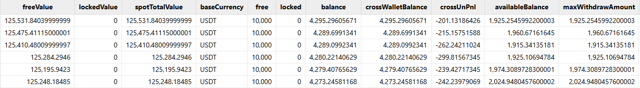
6.3 Risk Alert Notifications
This section explains how to implement real-time risk alerts via WeCom using the httpClient plugin, so you can be notified promptly. The implementation is similar to the real-time monitoring and alerting described in Chapter 2. The main alert function is shown below:
def sendWeChatMsg(msg, webhook){
    // JSON data
    sendcontent = dict(STRING, ANY)
    sendcontent["msgtype"] = "text"
    text = dict(STRING, STRING)
    text[`content] = msg
    sendcontent["text"] = text
    header = dict(STRING,STRING)
    header["Content-Type"] = "application/json"
    sendNum = 0   // for early warning, send once
    for(i in 1..5){
        if(sendNum != 1){
            try {
                jsontext = toStdJson(sendcontent)
                response = httpClient::httpPost(webhook, jsontext, 10000, header)
                sendNum = 1
            }catch (ex) {
                info = "send message " + webhook + " failed " + ex[1];
                writeLogLevel(WARNING, info);
            }
        }
    }
}- Select the chat group to receive alerts, create a notification bot, and obtain the webhook URL.
- Check the risk metric stream table. For example, if freeValue exceeds
12,500, send an
alert.
def checkRiskValueFunc(){ freeV = select * from objByName("portfolioRiskIndicatorST") order by updateTime desc limit 1 freeVal = freeV[`freeValue][0] if(freeVal > 12500){ msg = "Risk indicator freeValue is: " + freeVal + ". Please take action to control account risk." sendWeChatMsg(msg) } } - Schedule a task to check risk metrics every 10
minutes:
scheduleJob("checkRiskValue","check risk info",checkRiskValueFunc,09:00m+(0..18)*30,2025.09.12,2035.12.31,"D")
Using DolphinDB’s httpClient plugin, alerts can also be sent via email or other channels. For details, refer to the official documentation on integrating external messaging with the httpClient plugin.
7. Demonstration for More Strategies
Through three strategy examples (funding rate arbitrage, active market making, and dynamic grid trading), this section demonstrates how to write event callback functions using built-in DolphinDB scripts. Based on the existing cryptocurrency backtesting and simulation solution, it explains in detail how to use the DolphinDB’s cryptocurrency backtesting engine and rapidly implement strategies.
First, install and load the Backtest and httpClient plugins:
login("admin", "123456")
listRemotePlugins()          // View plugin repository
installPlugin("Backtest")    // Install plugin
installPlugin("httpClient")
loadPlugin("Backtest")       // Load plugin
loadPlugin("httpClient")
Based on the data environment prepared in Chapter 2, call CryptocurrencySolution::manageScripts. If strategy code management is required, declare the strategy name using module:
use CryptocurrencySolution::manageScripts
go
module cryptocurrencyStrategy   // Not required for backtest-only or simulation-only
7.1 Funding Rate Arbitrage Strategy
7.1.1 Strategy Overview
This section takes funding rate arbitrage as an example to show how to implement the strategy in the DolphinDB’s cryptocurrenct backtesting engine using minute-level market data. The arbitrage strategy profits from price differences across markets or assets. By buying and selling related assets at the same time, investors can lock in profits while hedging against price fluctuations.
Funding rate arbitrage is unique to the cryptocurrency market and originates from perpetual contract derivatives that are specific to cryptocurrency. The core idea is to go long or short perpetual contracts based on funding rate changes, while hedging with spot positions so that total portfolio value is insensitive to price movements (ignoring slippage and fees). The strategy logic is as follows:
- Short the contract: When the funding rate is greater than 0.03%, the market is bullish and longs pay funding fees to shorts. In this case, short the perpetual contract and buy an equivalent amount of the asset in the spot market. When the funding rate turns from positive to negative and the market trend changes, promptly close the contract position and sell the spot holdings.
- Long the contract: When the funding rate is less than −0.03%, the market is bearish and shorts pay funding fees to longs. In this case, go long on the perpetual contract and sell an equivalent amount of the asset in the spot market. When the funding rate turns from negative to positive and the market trend changes, promptly close the contract position and buy back the spot asset.
The following section implements only the short-side cryptocurrency perpetual contract strategy.
7.1.2 Strategy Implementation
The strategy initialization function initialize is triggered
only once after the engine is created, allowing you to set strategy
parameters. The parameter context represents the logical context.
Line 4 calls the setUniverse method to define the asset
universe and filter tradable assets. context["fundingRate"]
on line 5 is used to retrieve funding rate data for the backtest period,
while context["lastlastFunding"] on line 6 stores the
previous funding rate for use in the strategy to determine exit
conditions.
def initialize(mutable context){
    // Initialization
    print("initialize")
    // Backtest::setUniverse(context["engine"], context.Universe)
    context["fundingRate"] = Backtest::getConfig(context["engine"])[`fundingRate]
    context["lastlastFunding"] = dict(SYMBOL,ANY)  // Stores the previous funding rate, used to determine exit conditions
}
In the daily pre-market callback function beforeTrading, the
trading date can be obtained via context["tradeDate"], as
shown on line 4. In this example, the funding rate table for the current
trading day is converted into the d dictionary and passed into the strategy
through context. A nested dictionary structure is used, with the
symbol and the settlementTime as keys. The funding rate data is obtained in
the strategy initialization function.
def beforeTrading(mutable context){
    // Daily pre-market callback function
    // The current trading date can be obtained via context["tradeDate"]
    print("beforeTrading: " + context["tradeDate"])
    // Retrieve the funding rate table for the current day and store it as a dictionary keyed by symbol
    fundingRate = context["fundingRate"]
    d = dict(STRING,ANY)
    for (i in distinct(fundingRate.symbol)){
        temp = select * from fundingRate where symbol = i and date(settlementTime) = context["tradeDate"]
        replaceColumn!(temp, `settlementTime, datetime(exec settlementTime from temp))
        d[i] = dict(temp.settlementTime, temp.lastFundingRate, true)
    }
    context["dailyLastFundingPrice"] = d
}
In the OHLC data callback function onBar, the msg
parameter represents the latest minute-level market data passed in by the
backtest engine, and the parameter indicator represents the
subscribed provided by the engine. The code below demonstrates the logic for
determining entry and exit conditions.
def onBar(mutable context, msg, indicator = NULL){
    // ...
    dailyFundingRate = context["dailyLastFundingPrice"]
    // Iterate over multiple assets
    for(i in msg.keys()){
        istock = split(i,"_")[0]
        istockFut = istock + "_futures"
        istockSpo = istock + "_spot"
        source = msg[i]["symbolSource"]
        closePrice = msg[i]["close"]
        // Current asset funding rate; select the corresponding funding rate based on the current time window
        if(second(context["tradeTime"]) >= 16:00:00){fundingRateTime = temporalAdd(datetime(context["tradeDate"]), 16, "h")}
        if(second(context["tradeTime"]) >= 08:00:00 and second(context["tradeTime"]) < 16:00:00){fundingRateTime = temporalAdd(datetime(context["tradeDate"]), 8, "h")}
        if(second(context["tradeTime"]) < 08:00:00){fundingRateTime = datetime(context["tradeDate"])}
        lastFundingPrice = dailyFundingRate[istockFut][fundingRateTime]
        // print(fundingRateTime)
        // Position status: spot and futures
        spotPos = Backtest::getPosition(context["engine"], istockSpo, "spot")
        futurePos = Backtest::getPosition(context["engine"], istockFut, "futures")
        // ...
    }
}
Entry conditions are determined based on the funding rate and current
position size, and orders are placed via the
Backtest::submitOrder method.
// When the funding rate is greater than 0.03%, short the perpetual contract and buy an equivalent amount of spot
// Here the maximum order quantity is set to 0.1. To allow short-to-open, set 0.1 to 0.
if(spotPos.longPosition[0] <= 0.1 and futurePos.shortPosition[0] < 0.1 and lastFundingPrice > 0.0003){
    // Spot
    if(i == istockSpo){
        Backtest::submitOrder(context["engine"], (i, source, context["tradeTime"], 5, closePrice,
                  lowerLimit, upperLimit, qty, 1, slippage, 1, expireTime ), "buyopen_spot", 0, "spot")
    }
    // Contact
    if(i == istockFut){
        Backtest::submitOrder(context["engine"], (i, source, context["tradeTime"], 5, closePrice,
                  lowerLimit, upperLimit, qty, 2, slippage, 1, expireTime ), "sellopen_contract", 0, "futures")
    }
    context["lastlastFunding"][istockFut] = lastFundingPrice
}
Strategy execution:
strategyName = "cryptocurrencyStrategy"  // The code name must match the module name when storing
eventCallbacks = {
    "initialize": initialize,
    "beforeTrading": beforeTrading,
    "onBar": onBar
}
strategyType = 0  // Backtest — default is 10 days; start and end dates can be customized via userConfig
engine, straname_ = CryptocurrencySolution::manageScripts::runCryptoAndUploadToGit(strategyName, eventCallbacks, strategyType)
The userConfig parameter is set via the
getUnifiedConfig() function in the
CryptocurrencySolution::utils module by default. You
can customize it as follows:
userConfig = dict(STRING,ANY)
userConfig["startDate"] = 2025.12.01
userConfig["endDate"] = 2025.12.05
engine,straname_= CryptocurrencySolution::manageScripts::runCryptoAndUploadToGit(strategyName, eventCallbacks,strategyType,userConfig)
The full strategy script is provided in the Appendix.
7.2 Dynamic Grid Trading Strategy
7.2.1 Strategy Overview
This section illustrates how to implement a grid trading strategy based on minute-level market data in the cryptocurrency backtesting engine. Traditional grid trading strategies revolve around a reference price. When the price drops, buy at the trigger points; when the price rises, sell at the trigger points. This method is only suitable for small-range fluctuations. It struggles to capture upward trends during sudden large swings and cannot effectively avoid sharp declines. By reducing purchases during a crash and buying again once the market stabilizes, or by pausing sales during an uptrend and resuming once the trend slows, overall returns of the grid trading strategy can be improved.
The dynamic grid strategy define a grid spacing alpha and a rebound spacing beta. Trades are executed when the asset price first triggers a grid line and then reaches the rebound price. The logic is as follows:
- Construct grid strategy parameters: set the initial price as the first trade price of the strategy, grid spacing alpha as 2%, rebound spacing beta as 1%, and per-grid trade amount M as 100,000.
- Opening logic: when the asset price hits the n-th grid line below the reference price, wait for the latest price to rebound by beta from the lowest price, then buy a quantity of n * M / latest price.
- Closing logic: when the instrument price hits the n-th grid line above the reference price, wait for the latest price to fall by beta from the highest price, then sell a quantity of n * M / latest price.
- The reference price is updated to the latest buy or sell price according to the opening or closing signal.
7.2.2 Strategy Implementation
The strategy initialization function initialize is triggered
only once after creating the engine. You can set strategy parameters in
contextDict. The parameters lowPrice, highPrice,
baseBuyPrice, and baseSellPrice are used to update the
current reference prices.
def initialize(mutable contextDict){
    print("initialize")
    // Initial price
    contextDict["initPrice"] = dict(SYMBOL, ANY)
    // Grid spacing (percentage)
    contextDict["alpha"] = 0.01
    // Rebound spacing (percentage)
    contextDict["beta"] = 0.005
    // Trade amount per grid
    contextDict["M"] = 100000
    contextDict["baseBuyPrice"] = dict(SYMBOL, ANY)
    contextDict["baseSellPrice"] = dict(SYMBOL, ANY)
    contextDict["lowPrice"] = dict(SYMBOL, ANY)
    contextDict["highPrice"] = dict(SYMBOL, ANY)
    contextDict["N"] = dict(SYMBOL, ANY)
    // Fee rate
    contextDict["feeRatio"] = 0.00015
    Backtest::setUniverse(contextDict["engine"], contextDict.Universe)
}
Dynamic grid strategies need to update grid lines based on OHLC prices. A user-defined function is implemented as follows:
def updateBaseBuyPrice(istock,lastPrice,basePrice,mutable baseBuyPrice,mutable baseSellPrice,mutable N,mutable highPrice,mutable lowPrice,alpha,n,mode=0){
	// Update grid lines and highest/lowest price based on the latest price and base price
	baseBuyPrice[istock] = basePrice*(1-alpha)
	baseSellPrice[istock] = basePrice*(1+alpha)
	N[istock] = n
	if(mode==0){
		// Initialization for buy/sell, etc.
		lowPrice[istock]=0.
		highPrice[istock]=10000.
	}else if(mode==1){
		// Price drop, update lower grid line
		lowPrice[istock]=lastPrice
		highPrice[istock]=10000.

	}else if(mode==2){
		// Price rise, update upper grid line
		lowPrice[istock]=0.
		highPrice[istock]=lastPrice
	}
}
The OHLC callback function onBar receives msg, the
latest minute-level market data from the backtesting engine. The strategy
updates grid lines based on the latest price and base price in
contextDict. Trades are executed when the price hits
the upper or lower grid lines.
def onBar(mutable contextDict, msg,indicator){
	//...
    initPrice = contextDict["initPrice"]
    baseBuyPrice = contextDict["baseBuyPrice"]
	baseSellPrice = contextDict["baseSellPrice"]
    highPrice = contextDict["highPrice"]
    lowPrice = contextDict["lowPrice"]

	for(isymbol in msg.keys()){
		istock = isymbol
		lastPrice = msg[isymbol]["close"]
        source = msg[isymbol]["symbolSource"]
		// Set initial price
		if(not istock in initPrice.keys()){
			initPrice[istock]=lastPrice
			updateBaseBuyPrice(istock,lastPrice,lastPrice, baseBuyPrice,
			baseSellPrice, N, highPrice, lowPrice,alpha,1,0)
		}
		init_price=initPrice[istock]
		if(lastPrice<=baseBuyPrice[istock]){
			// Price drop, update lower grid line
			n=floor(log(lastPrice\init_price)\log(1-alpha))+1
			if(n>N[istock]){
				newBasePrice=init_price*pow((1-alpha),n)
				updateBaseBuyPrice(istock,lastPrice,newBasePrice,baseBuyPrice, baseSellPrice,
				N, highPrice, lowPrice,alpha,n,1)
			}
		}else if(lastPrice>baseSellPrice[istock]){
			// Price rise, update upper grid line
            //...
		}
		if(lowPrice[istock]>0. and lastPrice>lowPrice[istock]*(1+beta)){
			// Buy
			qty=decimal128(0.001,8)
			orderId = Backtest::submitOrder(contextDict["engine"], (istock, source, contextDict["tradeTime"],5, lastPrice,
			upperLimit, lowerLimit, qty,1, slippage, 1,expireTime ),"buy",0, "futures")
			initPrice[istock] = lastPrice
			updateBaseBuyPrice(istock,lastPrice,lastPrice, baseBuyPrice,
			baseSellPrice , N, highPrice, lowPrice,alpha,1,0)
		}else if(highPrice[istock]<10000. and lastPrice<highPrice[istock]*(1-beta)){
			// Sell ... (full code in attached script)
		}
		// Update lowest/highest price in real-time
		if(lowPrice[istock]>0){
			lowPrice[istock]=min([lowPrice[istock],lastPrice])
		}
		if(highPrice[istock]<10000.){
			highPrice[istock]=max([highPrice[istock],lastPrice])
		}
	}
    // Store updated prices
    contextDict["initPrice"]=initPrice
	contextDict["baseBuyPrice"]=baseBuyPrice
	contextDict["highPrice"]=highPrice
    //...
}
Strategy execution:
strategyName = "cryptocurrencyStrategy"  // Must match module name for code storage
eventCallbacks = {
	"initialize":initialize,
	"beforeTrading": beforeTrading,
	"onBar":onBar
}
strategyType = 0  // # Backtest – default 10 days; can customize start/end via userConfig
engine,straname_= CryptocurrencySolution::manageScripts::runCryptoAndUploadToGit(strategyName, eventCallbacks,strategyType)
The full strategy script is provided in the Appendix.
7.3 Active Market Making Strategy
7.3.1 Strategy Overview
Market-making strategies profit from the bid-ask spread and are a major approach in mid- to high-frequency trading. This section implements a classic Avellaneda-Stoikov (AS) market-making strategy on the BTC/USDT perpetual contract, demonstrating how to use DolphinDB to implement cryptocurrency strategies at snapshot frequency. The Avellaneda-Stoikov market-making model was proposed by Marco Avellaneda and Sasha Stoikov in their 2008 paper High-Frequency Trading in a Limit Order Book. The model studies how market makers set optimal quotes under inventory risk. Based on market price dynamics, the strategy considers price volatility, position, and risk preference. The AS model adjusts bid and ask quotes around the market mid-price to minimize inventory risk while maximizing profit.
The AS model derivation involves two steps. First, the market maker calculates the indifference price based on current inventory and risk preference. Second, by combining the quote’s distance from the market mid-price with market conditions and risk tolerance, the execution probability is estimated to determine the optimal quote. This approach allows market makers to provide liquidity while minimizing inventory risk and maximizing profit.
Indifference price formula:

 : market mid-price
 : market maker’s current inventory
 : market maker’s risk aversion
coefficient
: market maker’s risk aversion
coefficient : market price volatility
 : normalized end time
 : current time
This formula indicates that the larger the inventory or the higher the price volatility, the lower the market maker will set the mid-quote, reducing holding risk.
Spread formula:

 : symmetric bid-ask spread
 : same as the previous formula
 : market liquidity
This formula shows that a higher risk aversion, higher market volatility, or better market liquidity leads to a larger optimal spread for the market maker, compensating for risk.
Quote formula:


7.3.2 Strategy Implementation
The strategy initialization function initialize is triggered
once after the engine is created, allowing you to set strategy parameters.
The context parameter represents the logical context, while
userParam holds custom strategy parameters. In the AS strategy,
we directly input the preset values of the previously mentioned  for use in quote calculation.
def initialize(mutable context){
	print("initialize")
	Backtest::setUniverse(context["engine"], context.Universe)
	// Onsnapshot Parameters
    context["sigma"] = 0.025                                    // market volatility
    context["gamma"] = 0.1                                      // inventory risk aversion parameter
    context["k"] = 1.5                                          // order book liquidity parameter
    context["amount"] = 0.001                                    // order amount
    //...
	context["lastprice"] = NULL
	// Daily Trade Summary
	context['dailyReport'] = table(1000:0,
		[`SecurityID,`tradeDate,`BuyVolume,`BuyAmount,`SellVolume,`SellAmount,`transactionCost,`closePrice,`rev],
		[SYMBOL,DATE,DOUBLE,DOUBLE,DOUBLE,DOUBLE,DOUBLE,DOUBLE,DOUBLE])
}
In the snapshot callback function onSnapshot, the strategy
logic is mainly divided into seven steps:
- Use
orderIntervalas the order frequency—for example, check, calculate, and place orders every second. - Cancel existing orders before placing new ones.
- Calculate the current market mid-price from the best bid and ask.
- Retrieve the current long and short positions.
- Compute quotes based on the AS model. Note the decimal precision of the order price—for BTC/USDT, the minimum price increment is 0.1.
- Submit buy and sell orders.
- Manage inventory risk and close positions in a timely manner.
def onSnapshot(mutable context, msg, indicator){
	istock = context["istock"][0]
	if(context["lastprice"]<0){
		context["lastprice"] = msg[istock].lastPrice
	}
	// 1. Set frequency of each order
	t = msg[istock]["timestamp"]
	if(t < context["orderTime"]){return}
	context["orderTime"] = context["orderTime"] + context["orderInterval"]
	// 2. Cancel previous orders before submitting new one
	openOrders = Backtest::getOpenOrders(context["engine"],istock, , , "futures")
	if(count(openOrders)>0){
	Backtest::cancelOrder(context["engine"],istock)
	}
	// 3. Calculate Mid Price
	askPrice0 = msg[istock]["offerPrice"][0]
	bidPrice0 = msg[istock]["bidPrice"][0]
	midPrice = (askPrice0+bidPrice0)/2
	// 4. Get Position
	pos = Backtest::getPosition(context["engine"],istock,"futures")
	longPos = pos['longPosition']
	shortPos = pos['shortPosition']
	netPos = nullFill(pos['longPosition']-pos['longPosition'],0)
	if(count(netPos) == 0){
	    netPos = 0
	}
    // 5. Calculate order price
	gamma = context["gamma"]
	sigma = context["sigma"]
	k = context["k"]
	amount = context["amount"]
	endTime = timestamp(context["tradeDate"])
	timeToEnd = (endTime-t)\86400000
	reservePrice = midPrice - netPos * gamma * square(sigma) * timeToEnd
	spread = gamma * square(sigma) * timeToEnd + (2 / gamma) * log(1 + (gamma / k))
	buyPrice = reservePrice-0.5*spread
	sellPrice = reservePrice+0.5*spread
	buyPrice = round(buyPrice, 1)
	sellPrice = round(sellPrice, 1)
	// 6. Set order direction
	sellDirection = 3
	buyDirection = 4
	if(count(longPos) == 0 || longPos == 0){
	buyDirection = 1
	}
	if(count(shortPos) == 0 || shortPos == 0){
	sellDirection = 2
	}
	// 7. Submit buy orders
	Backtest::submitOrder(
	context["engine"],
	(istock, 'Binance', context["tradeTime"], 5, buyPrice,0, 1000000, amount, buyDirection, 0, 0, endTime),
	"buy", 0, "futures")
	// 8. Submit sell orders
	Backtest::submitOrder(
	context["engine"],
	 (istock, 'Binance', context["tradeTime"], 5, sellPrice, 0, 1000000, amount, sellDirection, 0, 0, endTime),
	"sell", 0, "futures")
}
In the strategy termination callback function finalize, you
need to implement order cancellation and post-trading log recording. An
example is as follows:
def finalize(mutable context){
	tradeDate = context["tradeDate"]
	print("afterTrading: "+tradeDate)
	// Cancel all open orders
	Backtest::cancelOrder(context["engine"],context["istock"][0])
	// AfterTrading Log
	tb = context["log"]
	context["log"] = tb.append!(table(context["tradeDate"] as tradeDate,now() as time,"afterTrading" as info))
}
Strategy execution
strategyName = "cryptocurrencyStrategy"  //When saving the code, the name must match the module name
eventCallbacks = {
	"initialize":initialize,
	"beforeTrading": beforeTrading,
	"onSnapshot":onSnapshot,
    "finalize":finalize
}
strategyType = 0  // Backtest — default is 10 days, but you can customize start and end time via userConfig
engine,straname_= CryptocurrencySolution::manageScripts::runCryptoAndUploadToGit(strategyName, eventCallbacks,strategyType)
The full strategy script is provided in the Appendix.
8. Writing Strategies with Swordfish
The high-frequency strategy backtesting engine in DolphinDB is implemented in C++. To improve backtesting performance, event callback functions can be implemented in C++ using Swordfish, enabling tight integration between C++ quantitative programs and DolphinDB. The architecture for calling backtesting plugin or DolphinDB function library from C++ via Swordfish is shown in Figure 8‑1.
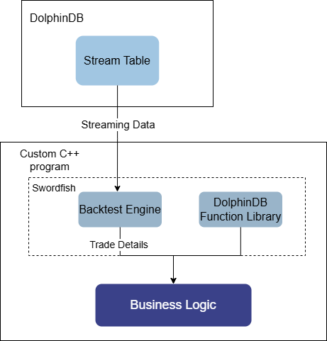
8.1 C++ Strategy Implementation
Taking a grid strategy as an example, this section explains how to use the backtesting plugin in C++ Swordfish.
Load the plugin:
Swordfish provides the DolphinDBLib::execute method to run
DolphinDB scripts. It returns a ConstantSP type, which is a pointer to the
Constant class and can be cast to the actual type. This method can call the
loadPlugin function to load the backtesting plugin,
returning an array of function pointers for all plugin methods. The type is
VectorSP, so the plugin can be loaded as follows:
VectorSP functions = DolphinDBLib::execute("loadPlugin('backtest')");To simplify the use of the backtesting plugin in C++, a demo in the Appendix wraps the DolphinDBLib::execute method into a BacktestWrapper class. Example:
auto engine = BacktestWrapper::createBacktester(strategyName_, userConfig_, eventCallbacks, new Bool(false), securityReference);Write the strategy:
When creating the backtesting engine, multiple strategy callback functions need
to be defined, and a dictionary mapping string keys to function pointers must be
passed to the eventCallbacks parameter of
createBacktester. The SwordfishFunctionDef class is
provided to convert C++ function pointers to Swordfish internal function
pointers. Example of defining the initialize callback function
for the backtesting engine:
ConstantSP initialize(vector<ConstantSP> &arguments) {
    cout << "initialize" << endl;
    DictionarySP contextDict = arguments[0];
    return new Void();
}

int main() {
    auto initializeFunc = new SwordfishFunctionDef(initialize, "initialize", 1, 1, false);
}
Constructor parameters of SwordfishFunctionDef:
- func:
const
                            std::function<ConstantSP(ddb::vector<ConstantSP>&)>
, a C++ function pointer type. It requires the input parameter to be of typeddb::vector<ConstantSP>&(a dynamic-length argument array) and returnsConstantSP. - name:
const std::string, the custom Swordfish function name. - minParamNum: int, minimum number of parameters.
- maxParamNum: int, maximum number of parameters.
- hasReturnValue: bool, whether the function has a return value.
onBar callback function. The arguments array
contains the logical context contextDict at index 0 and market
data msg at index
1:ConstantSP onBar(vector<ConstantSP> &arguments) {
cout << "onBar" << endl;
DictionarySP contextDict = arguments[0];
DictionarySP msg = arguments[1];
cout << "contextDict: " << endl << contextDict->getString() << endl;
cout << "msg: " << endl << msg->getString() << endl;
// ...
}Retrive data and run backtesting:
After creating the backtesting engine, connect to DolphinDB remotely to read market data and write it to the engine. The CryptoBacktest class is provided to implement the full backtesting workflow, offering the same runCryptoBacktest method as before. Example:
SmartPointer<DDBConnection> conn = new DDBConnection("192.198.1.32", 8742, "admin", "123456");
CryptoBacktest backtest(conn);
// ...
SmartPointer<BacktestWrapper> engine = backtest.runCryptoBacktest(strategyName, userConfig, eventCallbacks);
// Get backtesting results
cout << engine->getTradeDetails()->getString() << endl;
The full script is provided in SwordfishBacktest.zip in the Appendix, where the callback functions for the grid strategy are defined in main.cpp.
8.2 Python Swordfish Strategy Implementation
Python Swordfish is a high-performance embedded computation engine and database for Python users, introduced by DolphinDB. Unlike DolphinDB scripts, Python Swordfish embeds the database directly into the Python process, avoiding network transmission and serialization overhead, achieving maximum performance. Python Swordfish is deeply integrated with the Python ecosystem, making it suitable for quant teams that rely on Python tools.
Taking a grid strategy as an example, this section demonstrates the basic usage of the backtesting plugin in Python Swordfish.
Import Python Swordfish libraries
import swordfish as sf
import swordfish.plugins.backtest as backtest
import swordfish.function as F
Strategy template
The Swordfish libraries provides the StrategyTemplate class as a strategy template. You can create strategies by inheriting from this class. When placing orders, the self.submit_order method of this template class can be used. For details, refer to the Python Swordfish documentation or the Appendix.
import swordfish.plugins.backtest as backtest

class MyStrategy(backtest.StrategyTemplate):
    def initialize(self, context):
        pass
    def on_bar(self, context, msg, indicator):
        pass
Write strategy
In a grid strategy, the main logic is defined in the onBar
callback function. Strategy implementation is done in the MyGridStrategy
class.
class MyGridStrategy(backtest.StrategyTemplate, backtest.CryptoOrderMixin):
      #...
      # Dynamically update grid lines
      def updateBaseBuyPrice(self, context, isymbol, lastPrice, basePrice, n, mode):
          context["baseBuyPrice"][isymbol]=basePrice*(1-context["alpha"])
          context["baseSellPrice"][isymbol]=basePrice*(1+context["alpha"])
          context["N"][isymbol]=n
          if mode == 0:
              context["lowPrice"][isymbol]=0.0
              context["highPrice"][isymbol]=1000000.0
          elif mode == 1:
              context["lowPrice"][isymbol]=lastPrice
              context["highPrice"][isymbol]=1000000.0
          elif mode == 2:
              context["lowPrice"][isymbol]=0.0
              context["highPrice"][isymbol]=lastPrice

      def on_bar(self, context, msg, indicator):
          # ...
          for isymbol in msg.keys():
            lastPrice = msg[isymbol]["close"]
            if context["lowPrice"][isymbol] > 0 and lastPrice > context["lowPrice"][isymbol] * (1 + context["beta"]):
                # Buy condition
                qty = F.int(context["M"] / lastPrice)
                self.submit_order((isymbol, source, context["tradeTime"], 5, lastPrice,
                    upperLimit, lowerLimit, qty, 1, slippage, 1, expireTime), "buy", 0, AccountType.FUTURES)
                context["initPrice"][isymbol] = lastPrice
                self.updateBaseBuyPrice(context, isymbol, lastPrice, lastPrice, 1, 0)
            elif context["highPrice"][isymbol] < 1000000 and lastPrice < context["highPrice"][isymbol]*(1 - context["beta"]):
                # Sell condition
                # Check the position, and if the position is less than 0, do not sell.
                qty = F.int(context["M"] / lastPrice)
                self.submit_order((isymbol, source, context["tradeTime"], 5, lastPrice,
                    upperLimit, lowerLimit, qty, 3, slippage, 1, expireTime), "sell", 0, AccountType.FUTURES)
                context["initPrice"][isymbol] = lastPrice
                self.updateBaseBuyPrice(context, isymbol, lastPrice, lastPrice, 1, 0)
            # Update min and max prices
            if context["lowPrice"][isymbol] > 0:
                context["lowPrice"][isymbol] = F.min(context["lowPrice"][isymbol], lastPrice)
            if context["highPrice"][isymbol] < 1000000:
                context["highPrice"][isymbol] = F.max(context["highPrice"][isymbol], lastPrice)
Strategy configuration
The following code shows the basic configuration for a cryptocurrency minute-level strategy.
config = backtest.CryptoConfig() # Crypto strategy configuration
config.start_date = sf.scalar("2025.09.01", type="DATE")
config.end_date = sf.scalar("2025.09.10", type="DATE")
config.asset_type = backtest.AssetType.CRYPTO
config.cash = {
    AccountType.SPOT: 100000000.0,
    AccountType.FUTURES: 100000000.0,
    AccountType.OPTION: 100000000.0
}
config.commission = 0.00015
config.data_type = backtest.MarketType.MINUTE # Minute-level data
config.security_reference = sf.table(...) # Asset information
config.funding_rate = sf.table(...) # Funding rate information
backtester = backtest.Backtester(MyStrategy, config)
Input market data
Market data can be obtained via a DolphinDB connection or other data sources, and
then fed into the engine using the append_data method.
conn = sf.connect(host="192.168.100.43", port=8848, user="admin", passwd="123456")
sql = """
  select ... from loadTable(..)
"""
kline_data = conn.sql(sql)
backtester.append_data(kline_data)
Print backtesting results
After the backtest is complete, the results can be obtained using the following methods.
res = backtester.accounts[AccountType.FUTURES]
print(res.trade_details.to_pandas()) # Trade details
print(res.get_daily_position().to_pandas()) # Daily positions
print(res.daily_total_portfolios.to_pandas()) # Daily portfolio metrics
print(res.return_summary.to_pandas()) # Return summary
9. Appendix
Chapter 2
- Database and table creation: createDatabase.dos
- Historical and real-time data ingestion: Binance.zip, OKX.zip
- Real-time snapshot aggregation (trades + orders): depthTradeMergeScript.dos
- Real-time OHLC downsampling: klineMergeScript.dos
- Monitoring and post-market data backfilling: checkData.dos, getCleanKLineAfterDay.dos
- Funding rate data ingestion: Binance_fundingRate.dos, okx_fundingRate.dos,getLatestFundingRate.dos
- Visualization: real-timeCryptoMarketDataDashboard.json
Chapter 3
- State factor expression module: stateFactors.dos
- Daily batch factor computation: calfactor.dos
- Streaming factor computation: real_time_cal_factor.dos
- Factor database and table creation: createFactorDatabaseTable.dos
- Python environment dependencies: requirements.txt
- Model construction and training: Models.py
- Data preprocessing: DataPre.py
- One-click model loading: ModelsStruct.py
- Training examples for different models: LSTM_main.py, xgboost_main.py, LSTM_and_xgboost_main.py, transformer_main.py
- Backtesting demo based on stream tables: main.py, factorStrategy.dos, model.pth
- Backtesting demo based on real-time computation: demo.dos, test_LSTM.pth, test_LSTM_cpu.pth
Chapter 4
- Backtesting and simulation solution: CryptocurrencySolution.zip
- Backtesting and simulation data panel: Backtesting strategy dashboard.json, Simulation_strategy_dashboard.json
Chapter 5
- Live trading module: CryptocurrencyTrading.zip
- Live trading example: BinanceTradingDemo.dos, OkxTradingDemo.dos
- OKX signature function: hex2Base64-main.zip
Chapter 6
- Table creation: createTable.dos
- Risk metric computation: BinanceRiskInfo.dos, OKXRiskInfo.dos
Chapter 7
- Funding rate arbitrage strategy: funding_rate_arbitrage_strategy.dos
- Dynamic grid trading strategy: dynamic_grid_trading.dos
- Active market-making strategy: active_market-making.dos
Chapter 8
- C++ strategy implementation: SwordfishBacktest.zip
- Python swordfish strategy implementation: gridForCrypt.py