High-Performance Factor Evaluation with DolphinDB
In investment research, factors are central to explaining returns and asset pricing, and continuously validating and selecting effective factors is essential for achieving excess returns. Factor evaluation provides a standardized framework to assess both the statistical significance and the informational value of factors. This tutorial presents a high-performance factor evaluation framework built on DolphinDB, supporting analytical evaluation of both single-factor and two-factor models.
1. Introduction to Factor Evaluation Framework
Compared with Python-based solutions, DolphinDB delivers significantly higher data I/O efficiency in factor evaluation scenarios, providing a more efficient computational foundation for quantitative analysis. DolphinDB currently supports part of the functionality of the Alphalens module; however, the Alphalens project has long been discontinued and is costly to adopt in practice. Therefore, we aim to build a factor evaluation framework with improved readability and a more comprehensive set of evaluation metrics.
Relative to the existing Alphalens implementation in DolphinDB, the
factorBacktest module leverages metaprogramming (with macro
variables, requiring DolphinDB version 2.00.12 or later), which substantially
enhances code readability and structural clarity. The module evaluates factors using
the following core metrics:
| Category | Metric |
|---|---|
| drawdown | maximum drawdown |
| maximum excess return drawdown | |
| returns | annualized returns |
| annualized excess returns | |
| significance test of returns | |
| volatility | annualized volatility |
| annualized excess volatility | |
| Sharpe ratio | Sharpe ratio |
| information ratio | information ratio |
| relative win ratio | strategy outperformance ratio vs benchmark |
| information coefficient | mean information coefficient (IC) |
| standard deviation of IC | |
| proportion of IC > 0 | |
| proportion of IC > 0.03 | |
| mean rank IC | |
| rank ICIR |
The two modules differ in the following functionalities:
| Functionality | factorBacktest |
Alphalens |
|---|---|---|
| forward returns calculation for multiple holding periods | × | √ |
| factor return calculation | × | √ |
| factor turnover analysis | × | √ |
| strategy outperformance ratio vs benchmark | √ | × |
| Newey-West adjustment to correct for residual heteroskedasticity and autocorrelation | √ | × |
| Fama-Macbeth regression to adjust standard errors for cross-sectional residual correlation | √ | × |
| risk-adjusted factor returns | √ | × |
| dependent double sorts | √ | × |
After downloading the factorBacktest.dos file at the end of this document and
placing the module in the getHomeDir()+/modules directory, the
factorBacktest module can be accessed in DolphinDB. Using the
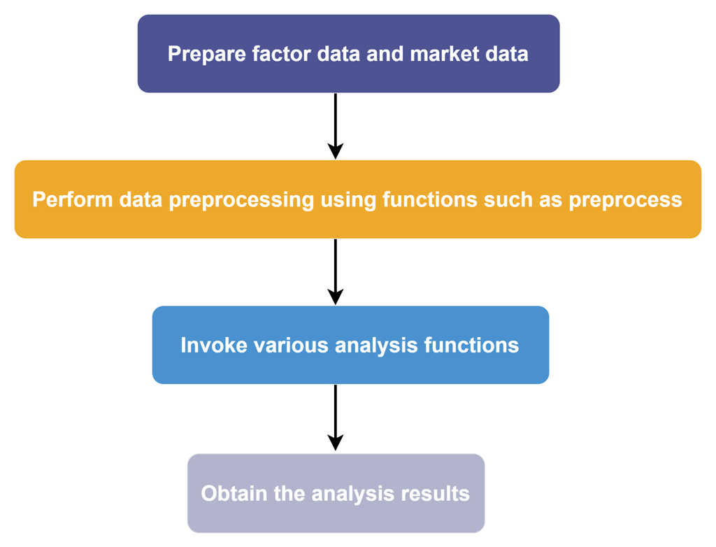
module typically involves four steps:
- Step 1: Prepare factor data and market data.
- Step 2: Perform data preprocessing using functions such as
preprocess. - Step 3: Invoke analysis functions.
- Step 4: Call the relevant functions to obtain the analysis results.
In the following sections, we will introduce how to use the
factorBacktest module step by step.
2. Data Preparation
2.1 Data Import
This factor evaluation framework uses the CSV files provided in the
factor_backtest_data directory. You can download the
factor_backtest_data archive from the end of this document and
extract it to <YOUR_DOLPHINDB_PATH>/server/. The data can then be
loaded directly with the loadText function for subsequent
computation and analysis.
factorTB = loadText("<YOUR_DOLPHINDB_PATH>/server/factor_backtest_data/factorTB.csv")
mktmvTB = loadText("<YOUR_DOLPHINDB_PATH>/server/factor_backtest_data/mktmvTB.csv")
industryTB = loadText("<YOUR_DOLPHINDB_PATH>/server/factor_backtest_data/industryTB.csv")
bp_factorTB = loadText("<YOUR_DOLPHINDB_PATH>/server/factor_backtest_data/bp_factorTB.csv")
bpTB = loadText("<YOUR_DOLPHINDB_PATH>/server/factor_backtest_data/bpTB.csv")
retTB = loadText("<YOUR_DOLPHINDB_PATH>/server/factor_backtest_data/retTB.csv")
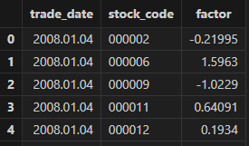
benchmarkTB = loadText("<YOUR_DOLPHINDB_PATH>/server/factor_backtest_data/benchmarkTB.csv")Use select top 100 * from factorTB to preview the factor in the
factorTB table, where trade_date is the trading date, stock_code is the stock
identifier, and factor is the factor name.
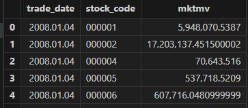
Use select top 100 * from mktmvTB to preview the market
capitalization in mktmvTB, where mktmv represents market capitalization of each
stock.
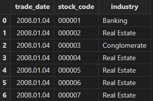
Use select top 100 * from industryTB to preview the industry
classification in industryTB, where industry indicates the industry of each
stock.
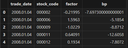
Use select top 100 * from bp_factorTB to preview the
multi-factor data in bp_factorTB, where both factor and bp are factor
variables.
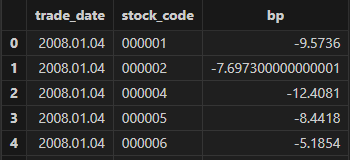
Use select top 100 * from bpTB to preview the bp factor in
bpTB.
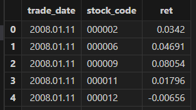
Use select top 100 * from retTB to preview the stock return in
retTB, where ret denotes returns.
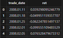
Use select top 100 * from benchmarkTB to preview the benchmark
return.
This module does not impose strict requirements on column names. You only need to ensure that the input tables follow the same schema as the examples above. For convenience, it is recommended to use consistent column names for trading dates and security identifiers across all input tables.
In terms of data frequency, the module supports input data at daily, weekly, or monthly frequencies.
2.2 Data Preprocessing
factor and bp can be processed directly using the
preprocess function, which performs outlier treatment,
standardization, and neutralization.
Code examples and a preview of the processed results are as follows:
use factorBacktest

//data preprocessing
factorNew = preprocess(factor=factorTB,
    factorName="factor",
    mktmvTB = mktmvTB,
    industryTB = industryTB,
    dateName = "trade_date",
    securityName = "stock_code",
    mvName = "mktmv",
    indName = "industry",
    delOutlierIf = true,
    standardizeIf = true,
    neutralizeIf = true,
    delOutlierMethod = "mad",
    standardizeMethod = "rank",
    n = 3,
    modify = false ,
    startDate = 2008.01.04,
    endDate = 2017.01.20)

// Observe the result after factor preprocessing
select top 100 * from factorNew

/*
 trade_date stock_code factor
 2008.01.04 000002 -0.06393232889798993
 2008.01.04 000006 1.5546531851632837
 2008.01.04 000009-1.2096673940460276
 2008.01.04 000011 0.7557481911404614
 2008.01.04 000012 0.32144219178486666
*/
The preprocess function exposes several key parameters:
- factorName: the name of the column that contains factor values in the input factor table. In the example, the factor values in factorTB are stored in the factor column.
- mvName and indName: the column names representing market capitalization and industry classification in the mktmvTB and industryTB tables, respectively.
- dateName and securityName: the column names for the trading date and the security identifier.
3. Single-Factor Analysis
The factorBacktest module provides a systematic and comprehensive
framework for single-factor analysis, enabling factor performance to be evaluated
from multiple perspectives. Key metrics include IC, ICIR, Rank IC, information
ratio, Sharpe ratio, and maximum drawdown, allowing for a thorough and well-rounded
assessment of factor effectiveness.
In this section, we use the factor extracted in the previous chapter as an example to
demonstrate how to perform single-factor analysis with the
factorBacktestmodule.
singleResult = singleFactorAnalysis(factorTB = factorNew,      //Factor data
    retTB = retTB,                               //Return table
    factorName = "factor" ,                      //Factor name
    nGroups = 5,                                 //Number of factor groups
    rf =0.0,                                     //Risk-free rate of return, default is 0
    mktmvDF = mktmvTB,                           //Market capitalization table
    dateName="trade_date",                       //Trading date column name
    securityName = "stock_code",                 //Security code column name
    retName = "ret",                             //Return column name
    mvName = "mktmv",                            //Market capitalization column name
    startDate = 2008.01.04,                      //start date
    endDate = 2017.01.20,                        //End date
    maxLags=NULL,                                //Lag order, default is NULL
    benchmark = benchmarkTB,                     //Market benchmark return table, default is NULL
    period = "DAILY" )                           //Frequency, valid values include "DAILY", "WEEKLY", "MONTHLY"
Single-factor analysis is conducted via the singleFactorAnalysis
function. The result singleResultis a dictionary with nine keys:
- groupRet: grouped portfolio return.
- retStat: statistical significance results for returns across groups.
- ICTest: calculations of IC, IR, and related metrics.
- backtest: grouped backtesting results for the factor.
- timeIndex: X-axis used for plotting.
- netValue: net asset value series of the grouped portfolios.
- retTable: long-short return series of the factor.
- title1 and title2: titles for the grouped net value curve and the long-short return curve, respectively.
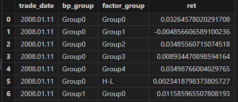
3.1 Grouped Returns
After preprocessing the factor data, stocks are sorted by factor values and divided into groups, and the return of each group is calculated. The "H-L" group represents the long-short portfolio return, calculated by going long on the highest factor group and short on the lowest factor group.
The grouped returns can be observed and formatted to six decimal places. An example of the corresponding code and results is shown below.
groupRet = singleResult["groupRet"]
groupname = ["Group0" , "Group1" , "Group2" , "Group3" , "Group4" , "H-L"]
<select top 10 trade_date , round(_$$groupname , 6)  as _$$groupname from groupRet>.eval()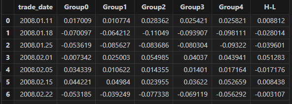
3.2 Statistical Significance of Grouped Returns
Once the grouped returns are calculated, their statistical significance can be tested. In multi-factor regression models, residuals often exhibit heteroskedasticity and autocorrelation. Using standard OLS to estimate the standard errors of β may lead to inaccurate results of significance testing. This module implements a Newey–West adjustment (Newey & West, 1987) to correct for heteroskedasticity and autocorrelation in the residuals.
The core Newey–West adjustment provides a consistent covariance estimator that corrects for heteroskedasticity and autocorrelation. Specifically:

- T denotes the total number of time periods,
- et is the residual at time t,
- Xi=[xi1,xi2,...,xiK]′ is the i-th row of X transposed,
- L is the maximum lag used to account for autocorrelation.
The resulting S is then substituted into the OLS variance expression VOLS to obtain the Newey–West heteroskedasticity- and autocorrelation-consistent covariance estimate.

In this section, the neweyWestTest function is used to estimate
the mean of grouped returns and output the t- and p-values adjusted via
Newey–West. The underlying computation is performed by the
neweyWestCorrection function.
The long-short portfolio statistics can be accessed via
singleResult["retStat"]["H-L"]. The output includes the
mean return (ret_mean(%)), p-value (p_value), and t-value (t_value).
// output:
// ret_mean(%): 0.465416325805543
// p_value: 0.00000568582996640643
// t-value: 4.591311581999794
Analyzing the above results, it can be seen that the mean long-short group return rate of the factor is 0.465%, the p-value is 0.0000056, and the t-value is 4.59, indicating that the mean long-short return rate is significantly different from 0.
3.3 IC Test
The information coefficient (IC) measures the cross-sectional correlation between factor values and next-period stock returns, and is commonly used to evaluate a factor’s predictive power. A larger absolute IC indicates a more effective factor. A positive IC implies that higher factor values are associated with higher future returns, while a negative IC suggests the opposite.
The information ratio (IR) is defined as the ratio of the mean excess return to its standard deviation, and reflects the stability of a factor’s ability to generate alpha.
By evaluating both IC and IR together, we can assess both the predictive strength and robustness of a factor, and determine whether it is reliable for sustained investment.
singleResult["icTest"]

/*
output:
Rank_ICIR: 0.10311019138174475
Rank_IC mean: 0.05030535697624222
IC mean: 0.03846492107792371
Factor name: 'factor'
IC standard deviation: 0.09652585561925417
IR: 0.39849344852894575
Proportion of IC>0 (%): 64.57883369330453
Proportion of IC>0.03 (%): 52.48380129589633
*/
The output obtained from singleResult["icTest"] is a dictionary
with eight keys. From the results, the IC mean is 0.038, which does not meet the
commonly accepted threshold for strong predictive power (≥ 0.05). The IR is
0.398, falling below the stability benchmark (≥ 0.5). Overall, the factor
exhibits only weak predictive ability and relatively poor stability.
In addition, the getFactorIc function can be used to plot both
time-series and cumulative charts of IC and Rank_IC. The corresponding code and
results are shown below.
correlation = getFactorIc(factorNew, retTB, "factor" ,"trade_date" ,"stock_code", "ret" , 2008.01.02 , 2017.01.31)
correlation['IC_cumsum'] = correlation["IC"].cumsum()
correlation['Rank_IC_cumsum'] = correlation["Rank_IC"].cumsum()
Observe the factor IC and Rank_IC results, and set the output format to six decimal places:
//Observe factor IC and Rank_IC results
groupname = ["IC" , "Rank_IC" , "IC_cumsum" , "Rank_IC_cumsum"]
<select top 10 trade_date , round(_$$groupname , 6)  as _$$groupname from correlation>.eval()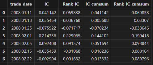
Plot using the plot function:
plot(table(correlation["IC"] ,correlation['IC_cumsum']) , correlation["trade_date"] , title = "FTime series plot and cumulative of IC for factor", extras={multiYAxes: true})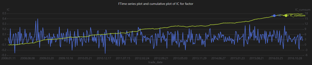
plot(table(correlation["Rank_IC"] ,correlation['Rank_IC_cumsum']) ,
              correlation["trade_date"] , title = "Factor factor Long-Short Return Curves (Market
              Cap Weighted)", extras={multiYAxes: true})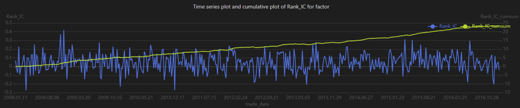
When analyzing IC time-series and cumulative charts, different types of information can be extracted. For example, frequent sign changes in IC, as shown in Figure 3-3, indicate unstable predictive performance across market regimes. The cumulative IC chart aggregates IC values over time and reflects the factor’s long-term predictive contribution. The steadily increasing cumulative IC in Figure 3-3 suggests that the factor consistently contributes positive expected returns over the long run.
3.4 Factor Analysis and Net Value Curves by Group
In this section, we analyze the backtest results for each factor-based portfolio
group and plot both the net value curves for the groups and the long-short
return curve. The results of the single-group factor analysis can be obtained
from singleResult["backtest"], as shown below.
backtestTB = singleResult["backtest"]
//Observe group backtest results
groupname = ["Group0","Group1","Group2","Group3","Group4","H_L","benchmark"]
<select index , round(_$$groupname , 6) as _$$groupname from backtestTB>.eval()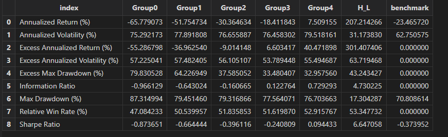
plot(singleResult["netValue"], singleResult["timeIndex"], singleResult["title1"])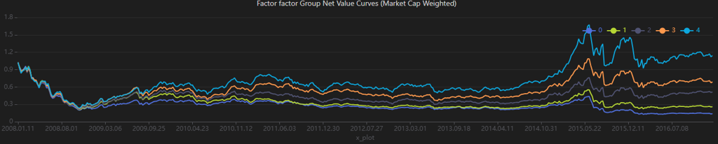
plot(singleResult["retTable"], singleResult["timeIndex"], singleResult["title2"])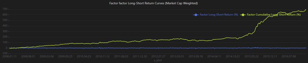
From the results, the factor demonstrates strong return differentiation across groups in the backtest. However, the relatively high volatility indicates weaker risk control. In comparison, the long-short strategy performs better, exhibiting lower volatility and higher returns.
4. Two-Factor Analysis
The factorBacktest module also supports two-factor analysis. In this
section, we use the factor and bp factors as examples to demonstrate
how to perform two-factor analysis with the factorBacktest
module.
doubleResult = doubleFactorAnalysis(factorTB1 = bpNew , //Factor table 1
    factorTB2 = factorNew, //Factor table 2
    retTB = retTB , //return table
    "bp" , //factor name 1
    "factor" , //factor name 2
    nGroups1 = 5, //Number of groups, default is 5
    nGroups2 = 5,
    mktmvTb = mktmvTB , //market capitalization table
    dateName ="trade_date" , //transaction date column name
    securityName = "stock_code", //Security code column name
    retName = "ret" , //Return column name
    mvName ="mktmv" , //Market capitalization column name
    startDate = 2008.01.04, //start date
    endDate = 2017.01.20, //Deadline
    maxLags = NULL, //Lag order, default is NULL
    rf=0.0 , //Risk-free interest rate, default set to 0
    benchmark =NULL, //Market benchmark return table, default is NULL
    period = "WEEKLY", //Frequency, optional parameters include "DAILY", "WEEKLY", "MONTHLY"
    regressionStep = false) //Boolean value, indicating whether to perform the first step of Fama-Macbeth regression calculation
The doubleFactorAnalysis function is used to obtain the analysis
results, where factorNew and bpNew are the results of factor and bp
factors after data preprocessing. The output doubleResult is a dictionary with 4
keys:
- dbSortRet: returns sorted jointly by the bp and the factor.
- dbSortMean: mean group returns along with Newey–West–adjusted t-statistics.
- dbSortBacktest: backtest results by factor group.
- famaMacbethResult: results from the Fama–MacBeth regression.
4.1 Returns from Dependent Double Sorts
In factor evaluation, dependent double sorts are commonly used to assess whether combining two factors leads to better performance than using either factor alone. This approach helps examine the degree of information overlap between the two factors and identify potential information again. Specifically, for two factors X and Y, assets are sequentially sorted and grouped by both factors to construct portfolios, whose performance is then analyzed.
4.2 Mean Returns from Dependent Double Sorts
After computing portfolio returns based on the dependent double sorts of the factor and bp factors, we further estimate the mean returns for each group and report the corresponding Newey–West–adjusted t-statistics. The relevant code and output are shown below.
dbSortMean = doubleResult["dbSortMean"]
groupname = ["Group0" , "Group1" , "Group2" , "Group3" , "Group4" , "H_L" ]
<select index , round(_$$groupname , 6) as _$$groupname from dbSortMean>.eval()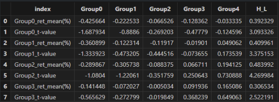
In the results table, the index column represents the bp-based groups. The Group0~Group4 columns denote the factor-based groups. The results show that:
- Across all bp groups, the H-L long-short returns are positive, with relatively high t-values, indicating that the high-factor portfolios significantly outperform the low-factor portfolios. This suggests that the factor consistently distinguishes asset returns across different bp groups.
- For each bp group, the mean returns generally exhibit an upward trend from Group0 to Group4. This suggests that higher bp groups are associated with improved portfolio performance across different factor groups, indicating a positive impact of the bp factor on returns.
- The factor shows stronger monotonicity and statistical significance among assets with medium to high bp values (e.g., Group3 and Group4), suggesting that the effectiveness of the factor is related to asset size characteristics.
4.3 Backtest Metrics for Dependent Double-Sorted Portfolios
The factorBacktest module also supports the computation of
backtest metrics for double-sorted portfolios. These results can be obtained
using doubleResult["dbSortBacktest"].
dbSortBacktest = doubleResult["dbSortBacktest"]
groupname = ["Group0" , "Group1" , "Group2" , "Group3" , "Group4" , "H_L" ]
<select index , round(_$$groupname , 6)  as _$$groupname from dbSortBacktest>.eval()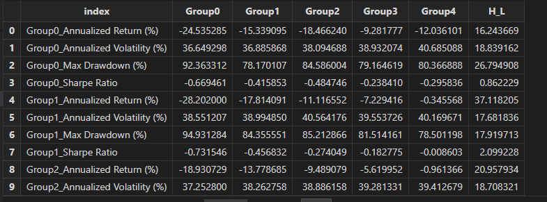
From the backtest metrics, we find that both the bp and factor values are positively associated with portfolio performance. As the bp and factor groups increase from Group0 to Group4, the Sharpe ratio and annualized returns rise steadily, while annualized volatility and maximum drawdown decline.
4.4 Fama–MacBeth regression
To mitigate the impact of cross-sectional correlation in regression residuals on
standard error estimation, the module also implements the Fama–MacBeth
regression based on Fama and MacBeth (1973), Risk, Return, and
Equilibrium: Empirical Tests. The functionality is provided
through the famaMacbethReg function.
Similar to conventional cross-sectional regression, the Fama–MacBeth approach consists of two stages.
In the first stage, a time-series regression is performed for each asset to estimate its factor exposure βi by regressing individual asset returns on the factor returns.

In the second stage, a cross-sectional regression is conducted at each time point t, where asset returns are regressed on their estimated factor exposures βi.

This step is repeated independently for every time point. For example, with T=500 time points, 500 cross-sectional regressions are performed, each using only the cross-sectional data at that time. The final regression coefficients are obtained by averaging the coefficients across all time points.


Since the coefficients from the second-stage regressions may exhibit heteroskedasticity and autocorrelation, Newey–West adjustments are applied to obtain consistent standard error estimates.
The Fama–MacBeth regression results can be accessed
viadoubleResult["famaMacbethResult"].
doubleResult["famaMacbethResult"]

/*
 output:
Average_Obs: 1,591.1749460043197
R-Square: 0.017901474327154446
factor:
   t-statistic: 6.986433993363168
   beta: 0.0019545565844644496
   p-value: 0.00000000000988853444
   standard error: 0.0002797645531785171
bp:
  t-statistic: 3.6404282777536614
  beta: 0.001105722959290441
  p-value: 0.00030294518028139983
  standard error: 0.0003037343067702823
*/
Note that the regressionStep parameter in famaMacbethReg
is a boolean vector indicating whether the two-step Fama–MacBeth procedure is
applied. By default, it is set to false, meaning that factor values are treated
as factor exposures (or factor exposures are directly provided), and only the
second-stage cross-sectional regression is performed.
The output is returned as a dictionary containing the model’s average R2, the average number of observations, and factor-specific statistics, including t-statistic, beta (risk premium), p-value, and standard error.
From the results, we observe the following:
- The model exhibits a relatively low R2, indicating limited explanatory power, with approximately 98% of the variation in asset returns not explained by the factor and bp factors.
- The factor has a statistically significant positive effect on asset returns, with an estimated risk premium of 0.00195.
- The bp factor also shows a statistically significant positive effect on asset returns, with an estimated risk premium of 0.00110.
5. Performance evaluation
In this section, we compare the performance of the DolphinDB and Python under the same factor backtesting framework. For identical tasks, both the data sources and computational results are kept consistent across the two implementations.
| Task | DolphinDB | Python |
|---|---|---|
| Data Preprocessing | 1.141 s | 3.867 s |
| Single-Factor Analysis | 1.117 s | 8.306 s |
| Two-Factor Analysis | 1.673 s | 11.970 s |
| Variable Name | Description | Size (rows × columns) |
|---|---|---|
| factorTB | raw factor table | 796,203 × 3 |
| factorNew | preprocessed factor table | 739,908 × 3 |
| bpTB | raw bp table | 964,744 × 3 |
| bpNew | preprocessed bp table | 957,733 × 3 |
| benchmarkTB | market benchmark return table | 463 × 2 |
| bp_factorTB | combined bp and factor table | 745,059 × 4 |
| industryTB | industry classification table | 1,069,702 × 3 |
| mktmvTB | market capitalization table | 974,754 × 3 |
| retTB | return table | 793,802 × 3 |
The results show that DolphinDB achieves faster execution across all tested scenarios compared with Python.
6. factorBacktest Function Reference
6.1 Utility Functions
| Function | Syntax | Description |
|---|---|---|
dropNullRow |
dropNullRow(table) |
Remove rows containing null values from the table |
getPreviousFactor |
|
Retrieve the factor values from the previous period |
6.2 Data Preprocessing Functions
| Function | Syntax | Description |
|---|---|---|
delOutlier |
|
Remove outliers from the factor values |
standardize |
|
Standardize the factor values |
neutralize |
|
Neutralize the factor values with respect to market capitalization and industry |
preprocess |
|
Perform preprocessing on the factor values, including outlier removal, standardization, and neutralization |
6.3 Core Performance Metric Functions
| Function | Syntax | Description |
|---|---|---|
maxDrawdownNew |
maxDrawdownNew(returns) |
Calculate the maximum drawdown, expressed as a percentage, defined as ( 1 - current net value / historical peak net value) |
annualizedReturn |
annualizedReturn(returns,
period="DAILY") |
Calculate the annualized return |
annualizedVolatility |
annualizedVolatility(returns,
period="DAILY") |
Calculate the annualized volatility |
annualizedSharpe |
annualizedSharpe(returns, rf=0,
period="DAILY") |
Calculate the annualized Sharpe ratio, defined as ( (annualized return - risk-free rate) / annualized volatility) |
erAnnualReturn |
erAnnualReturn(returns, benchmarkReturns,
period="DAILY") |
Calculate the annualized excess return, defined as ( (1 + annualized strategy return) / (1 + annualized benchmark return) - 1 ) |
informationRatio |
informationRatio(returns, benchmarkReturns,
period="DAILY") |
Calculate the information ratio, defined as annualized excess return divided by the standard deviation of excess returns |
winRate |
winRate(returns, benchmarkReturns) |
Calculate the relative win rate versus the benchmark |
6.4 Factor Analysis Functions
| Function | Syntax | Description |
|---|---|---|
getFactorIc |
|
Calculate the factor IC (information coefficient) time series |
neweyWestCorrection |
neweyWestCorrection(x, y, maxLags) |
Apply the Newey-West correction to account for autocorrelation and heteroskedasticity |
neweyWestTest |
neweyWestTest(arr, factorName="factor",
maxLags=NULL) |
Calculate the mean of returns and output the Newey-West adjusted t-statistic and p-value |
analysisFactorIc |
|
Perform single-factor IC analysis |
riskAdjAlpha |
|
Calculate risk-adjusted factor alpha and its t-statistic |
famaMacbethReg |
|
Perform Fama-MacBeth regression |
6.5 Grouping and Portfolio Construction Functions
| Function | Syntax | Description |
|---|---|---|
getStockGroup |
|
Sort stocks by factor values and assign them into groups |
getGroupRet |
|
Calculate the returns for each stock group |
getGroupRetBacktest |
|
Calculate backtest metrics for each group’s returns |
analysisGroupRet |
|
Perform single-group factor analysis |
getDoubleSortGroup |
|
Categorize stocks into dependent double-sorted groups |
getDoubleSortGroupRet |
|
Calculate returns for dependent double-sorted groups |
doubleSortMean |
|
Calculate the mean returns for dependent double-sorted groups |
doubleSortBacktest |
|
Calculate backtest metrics for dependent double-sorted groups |
7. Summary
In this tutorial, we use the factorBacktest module to implement a
clear and practical factor evaluation framework built on DolphinDB. It covers key
stages of the quantitative factor research workflow, including factor data
processing, return analysis, and backtest result evaluation, ensuring comprehensive
and reliable analytical outcomes. As such, it serves as a robust and efficient tool
for quantitative factor research.
The current factorBacktest module has certain limitations. For
example, it does not yet support return computations for varying holding periods.
Future versions will expand functionality and improve flexibility to better support
practical quantitative research workflows.
8. Appendix
- factorBacktest module source: factorBacktest.dos
- Sample data: factor_backtest_data.zip
- Performance comparison scripts:
- References