
Beginner’s Guide to Industrial Applications
1. Overview and Environment Setup
This tutorial is intended for users who are new to Internet of things (IoT). Using time-series data generated by industrial sensors as a running example, it explains how to use DolphinDB to build a basic IoT data processing and monitoring workflow that covers data modeling, data ingestion, query and analysis, real-time processing, and visual monitoring.
1.1 IoT Applications with DolphinDB
In IoT applications, we need to ingest, store, analyze, and process time-series data from large numbers of industrial sensors in real time. Such applications typically involve massive data volumes, high-frequency collection, and stringent real-time processing requirements. With its high-performance time-series database, distributed computing capabilities, and unified stream and batch processing architecture, DolphinDB has been widely adopted in industries such as energy and power, advanced manufacturing, scientific research, utilities, and fast-moving consumer goods.
-
Power industry: Monitor power generation equipment, analyze power grid operations and electricity trading, and manage smart meters to support equipment condition monitoring, fault alerts, and load analysis.
-
Advanced manufacturing: Collect industrial equipment data, monitor production lines, ensure quality traceability, manage equipment O&M, and analyze test data to improve production efficiency and equipment utilization.
-
Scientific research: Manage high-frequency data from large-scale experimental facilities and research equipment to support experimental data storage, trend analysis, anomaly tracing, and scientific computing.
-
Utilities: Monitor pipeline networks, analyze equipment operations, manage alerts, and optimize operations in industries such as water and gas utilities.
-
Fast-moving consumer goods: Monitor production equipment, manage cold-chain logistics, analyze warehouse operations, and optimize supply chains to ensure product quality and operational efficiency.
Typical IoT applications built with DolphinDB include unified device data ingestion, massive time-series data storage, real-time monitoring and alerting, equipment condition analysis, quality traceability, predictive maintenance, and data visualization. These capabilities help enterprises build a unified data analytics platform.
1.2 Environment Setup
Before you begin, download and deploy DolphinDB. Download the installation package from the DolphinDB Product Downloads page. For detailed deployment instructions, see Deployment. The examples in this tutorial use DolphinDB server 3.00.5 2026.02.06 LINUX x86_64 with a Community Edition license, running in standalone mode. You can run scripts and interact with the DolphinDB database through the web management interface, the VS Code extension, DolphinDB GUI, or a shell. In a production environment, you can scale to a distributed cluster based on data volume, write load, and query concurrency.
1.3 DolphinDB Architecture
As the number of devices, sampling frequency, and data retention period increase in IoT applications, systems typically require high-throughput writes, low-latency queries, parallel computing, and horizontal scalability. DolphinDB uses a shared-nothing distributed architecture in which each node has independent compute and storage resources. You can increase overall processing capacity by adding nodes.
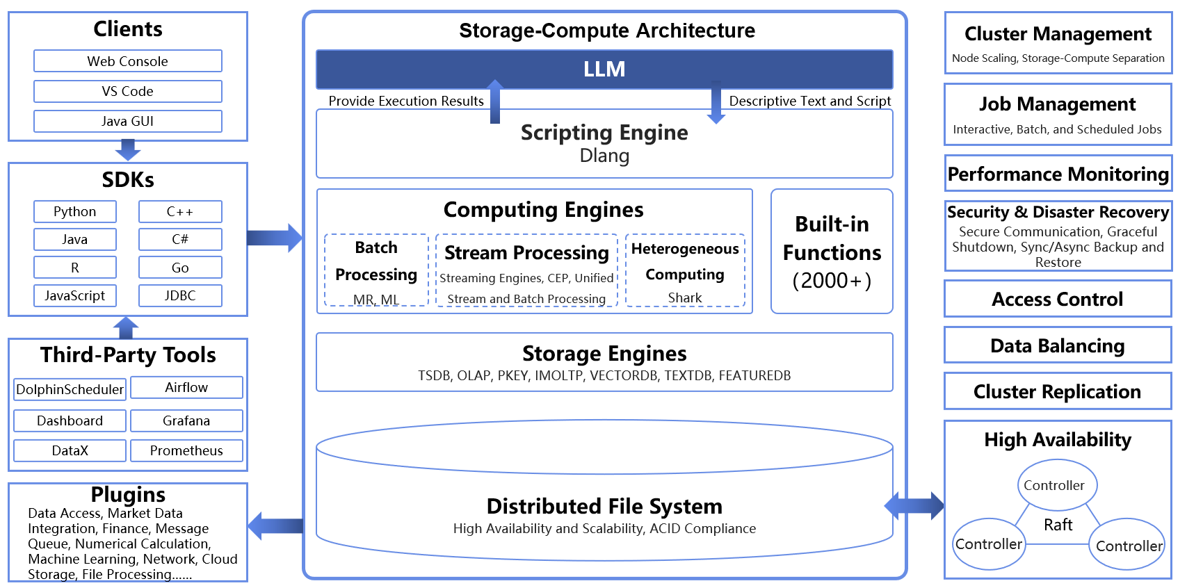
DolphinDB supports two operating modes: standalone and cluster. Standalone mode is suitable for learning in a local environment, feature validation, and small-scale trials. Cluster mode is designed for production environments and can support larger data volumes, heavier write loads, and higher query concurrency.
In cluster mode, DolphinDB typically consists of a controller, an agent, one or more data nodes, and one or more compute nodes. The controller manages cluster status, distributed file system metadata, and transaction logs. The agent receives instructions from the controller and starts or stops nodes. Data nodes store data and handle most query and computing tasks. Compute nodes process computations and queries without storing data, making them suitable for architectures that separate compute from storage.
For beginners, the roles can be summarized as follows: the controller manages the entire cluster, the agent starts and stops nodes, data nodes provide storage and computing, and compute nodes provide computing without storing data.
2. Data Modeling
This chapter uses a typical industrial sensor monitoring scenario as an example. Assume that a factory has 10,000 sensors deployed across different production lines and equipment. Each sensor reports data every 30 seconds, including temperature, pressure, humidity, voltage, current, and equipment status.
Estimated data volume:
-
Records reported by each sensor per day: 24×60×2=2,880
-
Records generated by 10,000 sensors per day: 2,880×10,000= 28.8 million
-
Each record is approximately 50 to 60 bytes, resulting in about 1.5 GB of raw data per day.
IoT data has two typical query patterns. The first retrieves historical data by device and time range, such as “Find the average temperature of device_0001 for all of yesterday.” The second retrieves the latest status of every device, such as “What are the current temperatures of all devices?” These two patterns directly affect the partitioning scheme and storage engine selection.
Why estimate the data volume first? Data volume determines the partitioning scheme, storage engine, and hardware resource configuration.
2.1 Table Schema Design
After determining the data volume, define the fields included in each reported record.
| Field Name | Data Type | Description | Design Rationale |
|---|---|---|---|
| device_id | SYMBOL | Device ID | Suitable as a HASH partitioning column and sort column, enabling efficient device-based queries |
| ts | TIMESTAMP | Data timestamp | Suitable as a time partitioning column, supporting time-range queries and window calculations |
| temperature | DOUBLE | Temperature | Numeric measurement suitable for aggregate analysis |
| pressure | DOUBLE | Pressure | Numeric measurement suitable for aggregate analysis |
| humidity | DOUBLE | Humidity | Numeric measurement suitable for aggregate analysis |
| voltage | DOUBLE | Voltage | Numeric measurement suitable for aggregate analysis |
| current | DOUBLE | Current | Numeric measurement suitable for aggregate analysis |
| status | INT | Device status | Suitable for statistics on discrete states, such as startup, shutdown, and alarm states |
Field Type Selection:
-
Time field ts: Use TIMESTAMP with millisecond precision and consistently name the field ts to facilitate time-range queries and window calculations.
-
Device ID device_id: Use the SYMBOL type. SYMBOL is DolphinDB's compressed string storage type. It is suitable for highly repetitive strings, such as device IDs, and can significantly reduce storage usage.
-
Numeric measurements: Use DOUBLE for values such as temperature and pressure to balance precision and storage efficiency. For metrics that do not require high precision, such as integer status values, use INT or FLOAT to reduce storage usage further.
-
Status field status: Use INT to facilitate grouped statistics and conditional evaluation.
Design principle: Base the schema on query conditions, write frequency, and field types. Plan the time, device ID, measurement value, and status fields together to avoid frequent schema changes later.
2.2 Selection Between Wide and Narrow Tables
In IoT applications, each device typically collects multiple sensor metrics, such as temperature, voltage, humidity, pressure, current, rotational speed, and status values. When modeling the data, decide whether to store these metrics in a single wide table, a narrow table, or multiple subject-specific tables.
| Evaluation Criterion | Better Suited to a Wide Table | Better Suited to a Narrow Table |
|---|---|---|
| Whether upload times are consistent | A device always reports multiple metrics together at the same timestamp | Metrics are reported at different frequencies and their timestamps do not always align |
| Whether the number of metrics is stable | The metric set is relatively fixed, with metrics rarely added or retired | Metrics are frequently added or retired, or their fields often change |
| Query patterns | Queries often retrieve multiple metrics by device and time, such as a device's temperature, voltage, and current over a specified period | Queries often retrieve data by metric, such as a specific metric across all devices |
| Data sparsity | Most metrics are included in every report | Many values are null for some metrics, resulting in clearly sparse data |
| Analysis patterns | Joint analysis of multiple metrics is common, such as correlation analysis among temperature, current, and pressure | Single-metric analysis is common, such as analyzing temperature or voltage trends independently |
The example in this tutorial assumes that each device reports metrics such as temperature, pressure, humidity, voltage, current, and status together at the same timestamp, and that the metric set is relatively stable. A wide table is therefore recommended. A wide table reduces the need for joins, improves read efficiency for queries by device and time range, and simplifies multi-metric aggregate analysis and status monitoring.
If your project includes many heterogeneous devices, frequently changing metrics, or substantial differences in sampling frequency across metrics, consider a hybrid model. For example, create a wide table for each device type, or store core metrics in a wide table and extended metrics in a narrow table. This approach balances query performance with model flexibility.
2.3 Storage Engine Selection
In DolphinDB, storage engine selection directly affects write performance, query efficiency, and compression ratio. OLAP, TSDB, and IOT are three storage engines commonly used in IoT applications. They address different requirements, ranging from offline analysis in traditional data warehouses to time-series data storage and querying. For descriptions of the OLAP, TSDB, and IOT storage engines, see the following tutorials: OLAP Storage Engine, TSDB Storage Engine, and IOT.
| Storage Engine | Indexing Mechanism | Query Patterns | Use Cases |
|---|---|---|---|
| TSDB | sortKey index + zone maps | Extremely fast queries by device and time, with efficient aggregation | General time-series monitoring and historical data queries |
| IOT | sortKey + latest-value cache | Millisecond-level response times for latest-value queries | Large-scale measurement management and high-frequency latest-value queries |
| OLAP | No independent index; relies on partition pruning | Efficient full table scans but slow point lookups | Traditional data warehousing and offline analysis |
TSDB improves time-series query efficiency through sort columns and partition pruning. It is well-suited to the requirements in this tutorial, including queries by device and time range, window aggregation, and status statistics. IOT is optimized for managing large numbers of measurements and querying the latest values, making it suitable for more advanced study. OLAP is better suited to traditional offline analysis and is not the preferred choice for the wide-table time-series data used in this tutorial.
2.4 Partition Design
The previous section selected the TSDB engine, but efficient TSDB queries also depend on an appropriate partition design. Even with the right engine, a poorly designed partitioning scheme can significantly degrade query performance. This section begins with the partitioning mechanism and progressively derives the partitioning scheme used in this tutorial to determine how to partition data for fast queries.
2.4.1 Partitioning Mechanism and Benefits
In DolphinDB's distributed architecture, DFS tables provide the primary means of storing massive data sets and performing parallel computation, while the partitioning mechanism is the foundation for organizing data in DFS tables. A DFS table generally refers to a table stored in a DFS database whose path begins with dfs://.
If all data is stored in a single large table, queries may need to scan a significant amount of irrelevant data. DolphinDB uses partitioning to divide a logical table into multiple physical partitions. During a query, it accesses only the matching partitions, reducing the amount of data scanned and improving query performance.
Partitioning a database provides the following key benefits:
-
Reduce the query scope: When query conditions match a partitioning column, only the relevant partitions are scanned, reducing I/O overhead.
-
Improve computational performance: Partitions can be distributed across multiple nodes, allowing queries and computational tasks to run in parallel.
-
Ensure high availability: Replicas can be configured for partitioned data, allowing data to be read from a replica if a node fails.
-
Support horizontal scaling: As data volume grows, you can add nodes to accommodate more partitions.
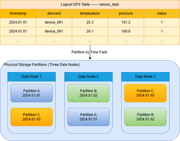
Figure 2-1 uses time-based partitioning to illustrate how logical partitions, replicas, and data nodes correspond to one another.
As shown above, the logical table sensor_data is partitioned by a time field. For example, the system writes data from January 1, 2025, to partition 2025.01.01 and maintains multiple replicas of the partition on different data nodes. If a data node fails, replicas of the partition remain available on other nodes. The system can continue reading from these replicas, ensuring continuous and highly available data access.
2.4.2 Partitioning Types and Selection
DolphinDB supports several partitioning types: range partitioning (RANGE), hash partitioning (HASH), value partitioning (VALUE), list partitioning (LIST), and composite partitioning (COMPO). For details, see Data Partitioning. The following three types are most common in IoT applications:
| Partitioning Type | Description | Use Cases |
|---|---|---|
| VALUE | Uses each unique value as a partition | Suitable for fields with low, fixed cardinality, such as dates |
| HASH | Uses a hash function to assign data to designated partitions | Suitable for high-cardinality fields with no clear distribution pattern, such as device IDs |
| COMPO | Uses two or three partitioning levels, each of which can use a different partitioning type | Suitable for large data volumes when queries frequently filter on multiple columns |
Composite partitioning is the preferred approach in DolphinDB for processing massive volumes of time-series data. It allows you to combine time and non-time dimensions in hierarchical partitioning. For example, you can use VALUE partitioning by date at the first level and HASH partitioning by device ID at the second level. This design uses time-based partitioning to quickly prune data by date range, while device-based HASH partitioning enables parallel writes and queries.
2.4.3 Partition Granularity and Data Volume Estimation
Due to the characteristics of a distributed architecture, partition granularity (the amount of data in each partition) has a significant impact on performance. You must strike a balance between partitions that are too large and those that are too small.
Problems caused by overly large partitions:
-
High I/O overhead during queries. Even when only a few records are required, the metadata for the entire partition may need to be read.
-
High memory pressure. DolphinDB must load partition metadata during queries, and overly large partitions may cause memory usage to exceed the license limit.
-
Maintenance difficulties. A partition is the smallest unit for operations such as compression and backup, so overly large partitions result in coarser maintenance granularity.
You can adjust partition granularity as follows:
-
To reduce partition granularity: 1. use COMPO partitioning; 2. increase the number of partitions; 3. replace RANGE partitioning with VALUE partitioning.
-
To increase partition granularity: 1. replace VALUE partitioning with RANGE partitioning; 2. reduce the number of hash buckets for HASH partitioning.
Problems caused by overly small partitions:
-
Queries span too many partitions, increasing inter-node communication overhead. In extreme cases, a single query may need to access tens of thousands of partitions.
-
Excessive metadata growth on the controller. Metadata for every partition must be registered with the controller. Too many small partitions can exhaust the controller's memory.
-
When too many partitions are involved, frequent reads and writes result in numerous inefficient disk accesses for small files, placing an excessive load on the system.
The following table lists the recommended partition sizes before compression:
| Storage Engine | Recommended Partition Size | Description |
|---|---|---|
| OLAP | 100-300 MB | Designed for analytical workloads and suitable for batch reads |
| TSDB | 400 MB-1 GB | A time-series engine that requires larger chunks to maximize compression benefits |
| IOT | 400 MB-1 GB | An IoT-specific engine similar to TSDB |
To estimate the total data volume, first estimate the size of a single row.
Estimate the row size from the number of bytes used to store each table field. Use the schema function to retrieve the data type of each table field. Then refer to Data Types for the number of bytes used by each type and add the field sizes together to estimate the size of a single row. The formula is: single-row data size = the sum of the bytes for each field type.
// Call the schema function to retrieve table field information (field name and type)
t.schema().colDefs

/*output:
name        typeString typeInt extra comment     sensitive
----------- ---------- ------- ----- ----------- ---------
device_id   SYMBOL     17            device ID   0
ts          TIMESTAMP  12            date        0
temperature DOUBLE     16            temperature 0
pressure    DOUBLE     16            pressure    0
humidity    DOUBLE     16            humidity    0
voltage     DOUBLE     16            voltage     0
current     DOUBLE     16            current     0
status      INT        4                         0*/
// Row size ≈ 4 (device_id) + 8 (ts) + 8 × 5 (5 DOUBLE metrics) + 4 (status) = 56 bytes
// Total storage: 28,800,000 rows × 56 bytes ≈ 1,612,800,000 bytes ≈ 1.5 GB
With daily partitions alone, each day would contain approximately 1.5 GB of data, approaching or exceeding the recommended partition size. Therefore, composite partitioning is required to reduce the amount of data in each partition. Use VALUE partitioning by date together with HASH partitioning by device ID to reduce partition size and improve parallel processing.
2.4.4 HASH Partition Planning
The number of HASH partitions must be specified when the database is created. Changing it later typically requires migrating or rewriting historical data. Therefore, plan the partition count at the beginning of the project based on the expected data growth over the next 1-3 years.
Calculations for This Tutorial:
| Parameter | Value |
|---|---|
| Daily data volume | 1.5 GB |
| Number of HASH partitions | 5 |
| Data volume per subpartition | 1.5÷5≈ 300 MB |
300 MB is slightly below the minimum recommended for TSDB (400 MB), but is still acceptable. If you choose 4 HASH partitions:
| Parameter | Value |
|---|---|
| Number of HASH partitions | 4 |
| Data volume per subpartition | 1.5÷4= 0.375 GB ≈384 MB |
With 4 HASH partitions, the data volume is close to the lower end of the recommended range. However, you must also account for future growth:
-
The current 10,000 devices may increase to 20,000 over the next 1-3 years.
-
If the data volume doubles, the data volume in each subpartition will also double: 384 MB×2= 768 MB, which remains within the recommended range.
-
If you allocate 5 partitions, doubling the data volume in the future gives: 1.5×2÷5= 600 MB, which is also within the recommended range.
Overall Recommendation:
| Number of Partitions | Current Size per Partition | After Data Volume Doubles | Assessment |
|---|---|---|---|
| 4 | 0.375 GB (384 MB) | 0.75 GB (768 MB) | Slightly below the recommended range now, but acceptable; performs well after future growth |
| 5 | 0.30 GB (300 MB) | 0.60 GB (600 MB) | Relatively small now, but more appropriately sized after future growth |
Either solution is suitable. This tutorial recommends allocating 4-5 HASH partitions. Choose the exact number based on your expectations for future data growth:
-
If you expect the number of devices to grow rapidly and double within 1-2 years, use 5 partitions.
-
If you expect more gradual growth, 4 partitions are sufficient.
Note: After the number of HASH partitions is specified at database creation, it cannot be changed directly. To change it, you must create a new database and table, then re-import the historical data. Therefore, make this decision upfront based on your business plans.
Final Partitioning Scheme for This Tutorial:
| Level | Partition Type | Partitioning Column | Number/Range of Partitions |
|---|---|---|---|
| First level | VALUE | ts (date) | One partition per day |
| Second level | HASH | device_id (device ID) | 4-5 (this tutorial uses 5) |
2.5 Database and Table Creation
The table creation syntax in DolphinDB SQL is similar to that of traditional SQL. In addition to specifying the table name, column names, and data types, you can also configure several database parameters. For details on using these parameters, see create.
create table dbPath.tableName (
    schema[columnDescription]
    // Column name Column type
    // [comment = Column description, compress = Compression method, index = Vector index]
)
[partitioned by partitionColumns], // Partitioning columns
[sortColumns], // Sort columns
[keepDuplicates=ALL], // Deduplication mechanism
[sortKeyMappingFunction] // Sort column mapping function
[softDelete=false] // Soft-delete configuration
[comment] // Table comment
Following the best practices for IoT sensor data, create the DFS table "sensor_data" in the database "dfs://iot_sensor". Use ts as the partitioning column for VALUE partitioning and device_id as the partitioning column for HASH partitioning. When data is written, the values in these partitioning columns determine how the data is divided and stored across partitions.
// Step 1: Create a composite-partitioned database
create database "dfs://iot_sensor"
partitioned by VALUE(2025.01.01..2025.01.03), HASH([SYMBOL, 5])
engine='TSDB'
// Step 2: Create a partitioned table
// The table schema includes the device ID, timestamp, temperature, pressure, humidity, voltage, current, and device status
// Partition by ts and device_id, and sort by device_id and ts to optimize queries
create table "dfs://iot_sensor"."sensor_data" (
    device_id SYMBOL[comment="device id"],
    ts TIMESTAMP[comment="date", compress="delta"],
    temperature DOUBLE[comment="temperature"],
    pressure DOUBLE[comment="pressure"],
    humidity DOUBLE[comment="humidity"],
    voltage DOUBLE[comment="voltage"],
    current DOUBLE[comment="current"],
    status INT
)
partitioned by ts, device_id
sortColumns=["device_id","ts"]
To design the database and tables through a graphical interface, see DolphinDB Web Interface: Database and Table Creation Guide. This tool allows you to configure partitioning schemes, field types, and sort columns without requiring any scripting knowledge.
2.6 FAQ
Q1: Is partitioning by year recommended?
In general, partitioning by year is not recommended. Partitioning by year can create excessively large partitions, reducing the efficiency of parallel queries, data migration, and maintenance. Even if your business archives data annually, partitioning the database by month or day is recommended. When a query spans multiple partitions, the system automatically merges the results.
Q2: Can the partitioning scheme be changed after it is created?
Because data storage depends on the partitioning scheme, you cannot modify the scheme directly. The best practice is to create a new database and table with the desired partitioning scheme, migrate the data, and then delete the original database and table.
-
Partitions can be appended: For VALUE partitioning, configure
newValuePartitionPolicy='add'to create partitions for new values automatically, or useaddValuePartitionsto add them manually. For RANGE partitioning, useaddRangePartitionsto append ranges. -
Partitioning rules cannot be modified directly: For example, changing the number of HASH partitions from 10 to 20 typically requires creating a new database and table and rewriting the historical data.
Q3: What should I check first when queries are slow?
Many factors can cause slow queries or writes. Troubleshoot the issue by examining the configuration, query or write patterns, database and table design, and system load. For details, see Slow Queries or Writes.
-
Check whether partition pruning is applied: The
WHEREclause should include partitioning columns. For example, for daily partitions, specify an explicit time range to avoid scanning irrelevant partitions. -
Check whether a single partition is too large: For TSDB and IOT engines, keep each partition between 400 MB and 1 GB. If a partition exceeds this range, add a second-level partition, such as HASH partitioning by device ID.
-
Check whether a full table scan occurs: Avoid
SELECT *without filters. Query only the required columns and narrow the scan range by applying common filters such as time and device ID.
2.7 References
-
DolphinDB Architecture: Distributed Architecture
-
Tutorial: Distributed Database Overview
-
Advanced Topics: TSDB Storage Engine
3. Data Ingestion
In IoT projects, data typically comes from gateways, sensors, business systems, message queues, or historical files. Because each source uses a different data pipeline, the ingestion methods also vary. The following table summarizes the methods for importing data into a DolphinDB database, the corresponding tools, and applicable scenarios. For details, see Data Import Method.
Table 3-1 Methods for Ingesting IoT Data into DolphinDB
| Ingestion Method | Typical Sources | Tools | Applicable Scenarios |
|---|---|---|---|
| Write via APIs | Gateway programs, edge services, and business applications | Write data through interfaces provided by APIs such as the DolphinDB C++ API, Python API, and Java API | Direct application writes with flexible development options |
| Ingestion via message queues | Kafka, MQTT brokers, IoT platforms, and similar systems | Ingest data through plugins for message queues such as Kafka and MQTT | Peak-load buffering and decoupling of producers and consumers |
| Synchronization via database plugins | MySQL, Oracle, SQL Server, and similar databases | Synchronize data through the MySQL and ODBC plugins | Existing data migration and synchronization across heterogeneous databases |
| File import | CSV, TXT, Parquet, and similar formats | Load data with the built-in text file loading functions loadText, ploadText, loadTextEx, and textChunkDS |
Offline batch processing and historical data migration |
The following sections use a simple sensor data table to demonstrate several ingestion methods.
3.1 Write via APIs
Writing data through APIs is one of the most widely applicable ingestion methods. It is suitable for gateway programs, edge services, business applications, and similar scenarios. Applications can collect, clean, and transform the data before calling a DolphinDB API to write it to the database. DolphinDB provides APIs for Python, Java, C++, Go, and other languages, making it easy to integrate with existing systems. For API-related tutorials, see API and Connector.
DolphinDB provides multiple API write methods for different data volumes and real-time processing requirements.
-
Single-row writes (insert into): Suitable for testing, validation, or low-frequency data scenarios. This method is simple to implement and easy to debug, but its low throughput makes it unsuitable for production environments.
-
Batch writes (tableInsert): Suitable for periodic uploads or writing device data in accumulated batches. This method reduces network overhead and provides good performance, but requires the client to buffer the data.
-
TableAppender: Suitable for low-frequency batch writes. It is easy to use, supports batch appends, and integrates seamlessly with existing scripts. However, throughput is limited, and you must manage the batch size yourself.
-
PartitionedTableAppender: Suitable for high-frequency, large-batch writes. It automatically routes data to partitions and takes full advantage of parallel writes across multiple partitions. To achieve optimal performance, however, you must configure appropriate partitioning columns and ensure that each batch is sufficiently large and spans multiple partitions.
-
MultithreadedTableWriter (MTW): Suitable for high-concurrency, high-throughput real-time IoT streams and continuous single-row writes that require consistently low latency. MTW significantly increases throughput through multithreaded parallelism, client-side buffering, and batch transmission. It also supports retrying failed writes and asynchronous callbacks, reducing per-row write overhead. However, you need to configure batchSize and the number of threads appropriately.
The following example generates a batch of simulated sensor data in Python and writes it in batches to a DolphinDB DFS table using tableInsert.
import dolphindb as ddb
import pandas as pd
# 1. Connect to DolphinDB
s = ddb.session()
s.connect("127.0.0.1", 8848, "admin", "123456")
# 2. Generate a batch of simulated data
data = pd.DataFrame({
    "device_id": ["dev001", "dev002", "dev003"],
    "ts": pd.to_datetime([
        "2025-01-01 10:00:00.001",
        "2025-01-01 10:00:00.002",
        "2025-01-01 10:00:00.003"
    ]),
    "temperature": [25.6, 26.1, None],
    "pressure": [101.3, None, 102.1],
    "humidity": [60.5, 58.2, None],
    "voltage": [None, None, 220.5],
    "current": [0.5, None, None],
    "status": [0, 1, 0]
})
# 3. Upload the DataFrame to the DolphinDB session
s.upload({"data": data})
# 4. Write the data to the DFS table in batches
s.run("""
pt = loadTable("dfs://iot_sensor", "sensor_data");
tableInsert(pt, data)
""")
print("write success")
When learning the basics or validating functionality, start with small-batch writes to make the workflow easier to understand and scripts easier to debug. In production, select accumulated batch writes, multithreaded concurrent writes, or asynchronous writes based on data volume and real-time requirements to improve throughput.
3.2 Ingestion via Message Queues
Message queues are commonly used as data channels for real-time IoT data ingestion. They decouple devices, gateways, and data platforms while improving system scalability, reliability, and the ability to handle traffic spikes. DolphinDB supports plugins such as Kafka and MQTT to subscribe to device messages and write the data to stream tables or DFS tables in real time, providing a complete pipeline from device data collection and message consumption to real-time analytics. For details, see Kafka and mqtt.
This tutorial uses Kafka to demonstrate how to subscribe to a Kafka topic with the Kafka plugin, parse device messages, and write the data to a stream table or DFS table, establishing a basic real-time ingestion pipeline.
The Kafka ingestion workflow consists of the following steps:
-
Load the Kafka plugin and configure the basic connection settings;
-
Create a Kafka consumer and specify the broker, consumer group, and offset policy;
-
Create a stream table to receive Kafka messages in DolphinDB;
-
Define a message parsing function that converts Kafka messages to the target table schema;
-
Subscribe to the Kafka topic and start the background consumption task;
-
Write the parsed data to the stream table and persist it asynchronously to the DFS table through a subscription task.
The following code is an example Kafka ingestion script. For the complete code, see the appendix: createKafka.dos
loadPlugin("kafka")

consumer=kafka::consumer(...)

kafka::subscribe(...)

kafka::createSubJob(...)
3.3 Synchronization via Database Plugins
Database plugins are primarily used to migrate or synchronize existing data from relational databases such as MySQL, Oracle, SQL Server, and PostgreSQL to DolphinDB for unified storage and analysis. Typical use cases include migrating device inventories, historical sample data, alert records, and transaction details, as well as periodically synchronizing incremental data.
DolphinDB provides mysql for connecting to MySQL and ODBC for connecting to Oracle, SQL Server, PostgreSQL, and other databases.
To use the ODBC plugin, first install the appropriate database driver and configure an ODBC data source name (DSN).
// 1. Load the ODBC plugin
loadPlugin("odbc")
// 2. Establish an ODBC connection
conn = odbc::connect("DSN=OracleDB;UID=iot_user;PWD=iot_password")
t = odbc::query(
    conn,
    "select device_id, ts, temperature, pressure, humidity,
    voltage, current, status from sensor_history
    where
    ts >= timestamp '2025-01-01 00:00:00'
    and
    ts < timestamp '2025-01-04 00:00:00'"
    )
t = select
    device_id$SYMBOL as device_id,
    timestamp(ts) as ts,
    temperature$DOUBLE as temperature,
    pressure$DOUBLE as pressure,
    humidity$DOUBLE as humidity,
    voltage$DOUBLE as voltage,
    current$DOUBLE as current,
    status$INT as status
    from
    t
// 4. Write to the DolphinDB DFS table
pt = loadTable("dfs://iot_sensor", "sensor_data")
tableInsert(pt, t)
The ODBC plugin provides a unified way to access multiple relational databases, making it a common solution for migration and integration across heterogeneous databases. In practice, pay attention to data type mappings. For example, Oracle types such as NUMBER, DATE, and TIMESTAMP must be mapped to the corresponding DolphinDB data types during import. Validate data type mappings and data quality with a small sample before performing a large-scale import.
3.4 File Import
File import is suitable for historical data migration, offline batch processing, data validation, and large-scale backfills. DolphinDB provides several functions for processing text files: loadText loads small files into an in-memory table for previewing and cleaning; loadTextEx imports large files directly into a DFS table without loading the entire file into memory; ploadText supports parallel loading; and textChunkDS processes extremely large files in chunks.
This tutorial demonstrates the process using loadText. This function is easy to use and creates a regular in-memory table after import. Before writing the data to a DFS table, you can use it to preview the data, inspect column types, add columns, or perform basic cleaning. It is therefore best suited for learning, testing, and small-scale data validation.
// Load a small CSV file into an in-memory table
data = loadText("/path/to/small_data.csv")
// Since the data has already been loaded into memory, it can also be validated before being written.
// View the data
select top 10 * from data
// View the column types
schema(data)
// Append the in-memory table to the DFS table
pt = loadTable("dfs://iot_sensor", "sensor_data")
tableInsert(pt, data)
3.5 FAQ
Q1: What should I do if I encounter a type mismatch when writing data?
First, check the column order and data types. For example, the device ID should be a STRING or SYMBOL, the sampled value should be a DOUBLE, and the sampling time should be a TIMESTAMP. A write may also fail if a time column in a Python DataFrame has not been correctly converted to a datetime type. For details, see PROTOCOL_DDB.
Q2: What should I do if API write performance is undesired?
Do not use insert into for high-frequency, single-row writes. Use batch tableInsert, PartitionedTableAppender, or MultithreadedTableWriter instead. Also verify that batchSize, the number of threads, and partitioning columns are configured appropriately.
Q3: What should I do if I cannot connect DolphinDB to Kafka or MQTT?
First, verify that the DolphinDB server can access the IP address and port of the Kafka broker or MQTT broker. Then check the username and password, topic name, consumer group, and network firewall settings.
Q4: What should I do if a file import fails?
First, check the file encoding, delimiter, column names in the header, and time format. For a large file, validate the first 100 rows before importing the complete file.
3.6 References
4. Data Query and Analysis
After data modeling and ingestion are complete, efficiently querying and analyzing the data becomes a key engineering concern. This chapter describes common DolphinDB query patterns and analysis methods for IoT applications, covering typical scenarios such as time-series queries, aggregate analysis, status monitoring, join queries, and data analysis.
The query examples in this chapter use the IoT use case from the data modeling chapter. The dataset contains 10,000 measurements collected from 2025.01.01 through 2025.01.03. Each measurement reports multiple metrics every 30 seconds, including temperature, pressure, humidity, voltage, current, and device status. This produces approximately 28.8 million records per day, making the dataset suitable for validation with DolphinDB Community Edition. For the simulated data, see genData.dos in the appendix.
The following sections explain how to implement common IoT statistical analysis requirements, helping you get started quickly with DolphinDB and address typical IoT analysis scenarios.
4.1 Basic Queries
4.1.1 Query by Device and Time Range
Query 100 records for "device_0001" on 2025-01-01. This query uses partition pruning to scan only the relevant partitions.
select
    *
from
    loadTable("dfs://iot_sensor", "sensor_data")
where
    device_id = 'device_0001'
    and
    ts
    between 2025.01.01T00:00:00.000
    and 2025.01.01T23:59:59.999
limit
    100
The preceding statement can also be written as follows:
select
    *
from
    loadTable("dfs://iot_sensor", "sensor_data")
where
    device_id = 'device_0001'
    and date(ts) = 2025.01.01
limit
    100
When time functions such as date and month are used as filter conditions on fine-grained temporal columns such as TIMESTAMP and DATETIME, DolphinDB automatically parses and optimizes the query. If the partitioning column is derived from a temporal field, this optimization can trigger partition pruning. As a result, the preceding query scans only the date partition for 2025.01.01. Combined with HASH partitioning on device_id, it can further narrow the scan to the corresponding device partition for that date, such as 2025.01.01/Key2. This syntax is more concise and intuitive, and is recommended for routine queries. The syntax in Method 1, which specifies the time range explicitly, is also valid. Choose either form based on your coding preferences.
4.1.2 Query the Latest Status
Retrieving the latest device status is a common requirement in real-time monitoring. DolphinDB provides the context by clause for window calculations, supporting operations such as sorting, applying functions, and selecting the top N records within each window.
select *
from loadTable("dfs://iot_sensor", "sensor_data")
context by device_id
csort ts desc
limit 1
The preceding query groups records by device_id, sorts each group by timestamp in descending order, and selects the first record from each group to retrieve the latest status of every device. The context by clause is a DolphinDB syntax extension that is more concise than traditional SQL window functions.
4.1.3 Cross-Sectional Queries
Query a cross-sectional time series of operating metrics for multiple devices over a specified time range to create a global view. The DolphinDB pivot by clause converts long-format data to wide format for easier side-by-side comparison.
select
    temperature,
    pressure,
    humidity
from
    loadTable("dfs://iot_sensor", "sensor_data")
where
    ts between 2025.01.01T00:00:00.000
    and 2025.01.01T00:01:00.000
    and device_id between "device_0001"
    and "device_0100"
pivot by ts,device_id
The pivot by clause preserves the time dimension based on ts and expands device_id values into columns, converting the long table into a wide table suitable for side-by-side comparison. The result makes it easier to visualize the cross-sectional status of multiple devices over the same period in tools such as Grafana. It also simplifies pivot analysis of time-series data. When pivot by is used with exec, the query returns a matrix, which is suitable for calculating analytical metrics such as correlations or similarities across multiple devices in batches.
Note: Cross-sectional device analysis can generate wide tables with many columns and large volumes of data. In the where clause, restrict both the time range and device range to query only the devices of interest. This prevents excessive cross-sectional data from being returned at once, which can cause long rendering times in front-end tools such as VS Code and web clients.
4.2 Aggregate Analysis
Raw IoT data is typically generated continuously at second-level or subsecond frequencies. Querying and analyzing detailed data directly often incurs substantial storage scan and computation costs. Aggregate analysis uses downsampling and statistical calculations to significantly reduce data volume while preserving overall trends and key features. This supports downstream scenarios more efficiently, including time-based curve monitoring, device reporting statistics, and machine learning model training.
4.2.1 Time-Window Aggregation
Downsampling aggregates high-frequency raw data into lower-frequency statistics and is commonly used to generate trend charts or reports. The bar function aligns timestamps to a specified interval and works with aggregate functions to downsample data.
The following example calculates the average temperature and maximum humidity for each device at 10-minute intervals:
select
    device_id,
    ts_bar,
    avg(temperature) as temp_avg,
    max(humidity) as humidity_max
from
    loadTable("dfs://iot_sensor", "sensor_data")
where
    ts between 2025.01.01T00:00:00.000
    and 2025.01.01T00:59:59.999
group by
    device_id,
    bar(ts, 10m) as ts_bar
bar(ts, 10m) assigns timestamps to 10-minute time buckets. Because the sample data spans one hour, a 10-minute window produces six data points for convenient observation. This pattern is suitable for generating minute-level, hourly, and daily trend reports.
In addition to the bar function, DolphinDB provides the interval function for time-window aggregation. The interval function is particularly useful in IoT scenarios because it can fill missing values through interpolation, allowing it to handle irregular device reporting intervals or missing data. For example, if a network outage prevents a device from reporting data for several minutes, interval can automatically fill the missing values or apply linear interpolation to maintain continuity in the aggregated results.
select device_id,
       ts,
       avg(temperature) as temp_avg,
       max(humidity) as humidity_max
from
      loadTable("dfs://iot_sensor", "sensor_data")
where
      date(ts) = 2025.01.01
group by
      device_id,
      interval(ts, 1m, "prev") as ts
For details about the interval function, including fill modes and boundary handling, see interval.
4.2.2 Full-Data Aggregate Statistics
Full-data aggregation analyzes the statistical characteristics of the entire dataset. The following example calculates the average temperature, maximum pressure, and minimum voltage across all devices within a specified time range:
select
    nunique(device_id) as device_count,
    avg(temperature) as avg_temperature,
    max(pressure) as max_pressure,
    min(voltage) as min_voltage,
    avg(current) as avg_current
from
    loadTable("dfs://iot_sensor", "sensor_data")
where
    date(ts) = 2025.01.01
nunique is equivalent to count(distinct…).
4.2.3 Moving-Window Calculations
Moving-window calculations analyze local trends in metrics, such as moving averages and moving standard deviations.
Traditional SQL implements moving windows with the OVER clause:
select
    device_id,
    ts,
    temperature,
    avg(temperature) over (
        partition by device_id
        order by
            ts rows between 10 preceding
            and current row
    ) as moving_avg
from
    loadTable("dfs://iot_sensor", "sensor_data")
where
    date(ts) = 2025.01.01
limit
    100
DolphinDB provides built-in moving window functions with more concise syntax:
select
    device_id,
    ts,
    temperature,
    mavg(temperature, 10) as moving_avg_10
from
    loadTable("dfs://iot_sensor", "sensor_data")
where
    date(ts) = 2025.01.01
context by
    device_id csort ts
limit
    100
mavg(temperature, 10) calculates a 10-point moving average over the current record and preceding records, helping smooth short-term fluctuations and reveal temperature trends. DolphinDB provides a comprehensive set of built-in moving window functions, including mavg, msum, mmax, mmin, and mstd. You can apply these functions directly to ordered sequences grouped by the context by clause and configure a different window size for each metric. This eliminates lengthy OVER clauses and provides concise syntax for analyzing trends and identifying anomalous fluctuations in IoT time-series metrics.
For more information about window calculations, see Window Calculations.
4.3 Status Analysis
In industrial applications, device status monitoring and safety threshold alerts are core features of O&M systems. This section explains how to use SQL to address common requirements such as calculating device uptime and downtime, generating out-of-limit alerts, and detecting idle operation.
4.3.1 Calculate Cumulative Uptime and Downtime
Cumulative device uptime and downtime are key metrics for full lifecycle management. Assume that status = 1 indicates that the device is on, while 0 indicates that it is off.
The calculation works as follows: Use bar(ts, 10m) to group the data into 10-minute intervals, further group it by device status, and then sum the differences by device within each time and status group to obtain the cumulative duration.
select
    device_id,
    status,
    ts,
    sum(duration_ms) / 60000.0 as duration_minutes
from
    (
        select
            device_id,
            ts,
            status,
            iif(isNull(next(ts)), 0, next(ts) - ts) as duration_ms
        from
            loadTable("dfs://iot_sensor", "sensor_data")
        where
            device_id = "device_0001"
        and
            date(ts) = 2025.01.01
        context by
            device_id
        csort
            ts
    )
group by
    device_id,
    status,
    bar(ts, 10m) as ts
4.3.2 Count Startups and Shutdowns
Count device startups and shutdowns within a specified period to assess how frequently each device is used.
The calculation works as follows: Use the deltas function to calculate the difference between adjacent status values. A difference of 1 indicates a transition from off to on, while a difference of -1 indicates a transition from on to off. Count the records with differences of 1 and -1 to obtain the startup and shutdown counts.
select
    device_id,
    sum(iif(deltas(status) == 1, 1, 0)) as start_count,
    sum(iif(deltas(status) == -1, 1, 0)) as stop_count
from
    loadTable("dfs://iot_sensor", "sensor_data")
where
    device_id = 'device_0001'
and
    date(ts) = 2025.01.01
group by
    bar(ts, 10m),
    device_id
The iif function applies conditional logic so that only records containing a status change are counted.
4.3.3 Obtain Maximum Continuous Operating Time
The maximum continuous operating time reflects a device's ability to operate reliably and is an important metric for predictive maintenance.
The calculation works as follows: Use deltas to calculate timestamp differences. Use the segment function to group records by status, placing consecutive records with the same status in one group. Filter for groups in which the device is on (1), calculate the duration of each group, and take the maximum as the maximum continuous operating time.
select
    device_id,
    max(running_duration) / 1000 as max_running_sec
from
    (
        select
            device_id,
            sum(iif(status == 1, deltas(ts), 0)) as running_duration
        from
            loadTable("dfs://iot_sensor", "sensor_data")
        where
            date(ts) = 2025.01.01
        group by
            device_id,
            segment(status)
    )
group by
    device_id
The segment(status) function generates a new group identifier whenever the status value changes, grouping consecutive on or off records together.
4.3.4 Query Threshold Violation Alerts
Threshold violation alerts detect whether sensor data exceeds safe operating limits. The following example queries anomalous records in which the temperature is above 80 degrees or below 20 degrees:
select
    device_id,
    ts,
    temperature
from
    loadTable("dfs://iot_sensor", "sensor_data")
where
    date(ts) = 2025.01.01
    and (
        temperature > 80
        or temperature < 20
    )
For rate-of-change alerts, such as detecting sudden current changes, use ratios to calculate the ratio between adjacent values:
select
    *
from
    (
        select
            ts,
            device_id,
            current,
            ratios(current) - 1 as changePct
        from
            loadTable("dfs://iot_sensor", "sensor_data")
        where
            device_id = 'device_0001'
            and date(ts) = 2025.01.01
    ) t
where
    abs(t.changePct) > 1
The preceding query detects anomalous data with a rate of change greater than 100%.
4.3.5 Obtain Idle Time
A device is considered idle when it is running with no workload or a very low workload. This state is typically identified using a current threshold, such as current < 20.
The calculation works as follows: Filter for records in which the current is below the threshold, use deltas to calculate the duration of the idle state, and aggregate the results by time window.
select
    device_id,
    sum(deltas(ts)) / 60000 as no_load_minutes
from
    loadTable("dfs://iot_sensor", "sensor_data")
where
    device_id = 'device_0001'
    and current < 20
    and date(ts) = 2025.01.01
group by
    bar(ts, 10m),
    device_id
4.4 Multi-Table Joins
IoT data analysis often requires joining device metadata or data from multiple sensors to provide more complete contextual information.
Device metadata, such as device names, locations, and models, is typically stored in a separate table and must be combined with sensor data through join queries. Assume that a device metadata table named device_metadata contains device location information:
// Create a device metadata table (in-memory table example)
device_list = "device_" + string(1..10000).lpad(4, "0")
device_metadata = table(
    device_list as id,
    take(["Factory_A", "Factory_B", "Factory_C"], 10000) as location,
    take(["Type_A", "Type_B"], 10000) as device_type
)
// Join query: retrieve data for devices located at Factory_A
select
    d.location,
    s.device_id,
    s.temperature,
    s.ts
from
    loadTable("dfs://iot_sensor", "sensor_data") s
    inner join device_metadata d on s.device_id = d.id
where
    d.location = 'Factory_A'
    and date(s.ts) = 2025.01.01
In addition to inner joins, DolphinDB supports common left, right, outer, semi, and full joins, as well as extended join syntax such as window join, asof join, and prefix join.
4.5 FAQ
Q1: How do I resolve mismatched temporal types?
DolphinDB supports multiple temporal types, including DATE, DATETIME, TIMESTAMP, and MINUTE. Values of different temporal types cannot be compared directly. If SQL execution returns the error “Temporal data comparison should have the same data type”, convert the values to the same type.
-- Method 1: Use a temporal conversion function
select
    *
from
    loadTable("dfs://iot_sensor", "sensor_data")
where
    date(ts) = 2025.01.01
limit
    10
-- Method 2: Use a full timestamp string of the corresponding type
select
    *
from
    loadTable("dfs://iot_sensor", "sensor_data")
where
    ts
    between 2025.01.01T00:00:00.000
    and 2025.01.01T23:59:59.999
limit
    10
Q2: How can I optimize query performance?
SQL query performance depends on two key factors:
Partition pruning: Ensure that query conditions include the partitioning columns so that the system can exclude irrelevant partitions. For a table partitioned by time and device hash, specify both a time range and a device identifier in the query.
Index utilization: Query performance in the TSDB engine depends on indexes for the sort columns. Query conditions should include the leading sort columns so that the index can be used to locate the data.
-
Partition Pruning
Add [HINT_EXPLAIN] to the SQL statement to obtain the execution plan. The "partitions" property in the plan shows the number of partitions scanned by the query engine.
select
    [HINT_EXPLAIN] *
from
    loadTable("dfs://iot_sensor", "sensor_data")
where
    date(ts) = 2025.01.01
The "partitions" property in the preceding SQL execution plan shows that five partitions were accessed: the five hash partitions under the 2025.01.01 partition, with paths in the form 20250101/Key2/z. The where date(ts) = 2025.01.01 condition causes the query engine to access only the 2025.01.01 partition instead of all partitions from 2025.01.01 through 2025.01.03.
{
    "measurement": "microsecond",
    "explain": {
        "from": {
            "cost": 16
        },
        "map": {
            "partitions": {
                "local": 5,
                "remote": 0
            },
            "cost": 90424,
            "partitionRoute": {
                "local8848": 5
            },
            "detail": {
                "most": {
                    "sql": "select [253967] device_id,ts,temperature,pressure,humidity,voltage,current,status from sensor_data [partition = /iot_sensor/20250101/Key9/3cj]",
                    "explain": {
                        "rows": 35700,
                        "cost": 78764
                    }
                },
          //Skip other information
    }}}
}-
Index Utilization
When the where clause includes the indexed column (device_id), the query engine can use the TSDB engine's index for fast lookups, significantly reducing the number of blocks scanned.
select [HINT_EXPLAIN] * from loadTable("dfs://iot_sensor", "sensor_data")
where date(ts) = 2025.01.01 and device_id = "device_0001"
The execution plan includes the "TSDBIndexPrefiltering" property. matchedWhereConditions=1 indicates that the engine performed an index lookup based on the where condition.
"where": {
            "TSDBIndexPrefiltering": {
                "blocksToBeScanned": 7,
                "matchedWhereConditions": 1
            },
            "rows": 300,
            "cost": 4105
}
The following SQL statement cannot effectively use sortKey and should be avoided.
select [HINT_EXPLAIN] * from loadTable("dfs://iot_sensor", "sensor_data")
where date(ts) = 2025.01.01 and substr(device_id, 7, 4) = "0001"
Its execution plan changes to the following:
"where": {
    "TSDBIndexPrefiltering": {
        "blocksToBeScanned": 651,
        "matchedWhereConditions": 0
    },
    "rows": 0,
    "cost": 12621
}
Its execution time increases from 5 ms to 50 ms. In a production environment, the performance difference in latency, I/O, and memory consumption can be even greater.
4.6 References
This chapter systematically introduced common data query and analysis techniques for IoT scenarios, including time-series queries, aggregate statistics, status monitoring, join analysis, trend analysis, and query performance optimization. For more information about SQL development techniques and performance analysis methods, see the following document:
-
Analyzing SQL execution plans: SQL Execution Plan
5. Real-Time Computing
Industrial IoT applications require real-time processing capabilities such as second-level aggregation of device metrics, immediate anomaly detection, and control command triggering. Conventional approaches based on database polling or Kafka+Flink can introduce high latency, impose heavy system loads, or require a complex technology stack. DolphinDB provides a unified stream processing framework that manages data through stream tables. It offers ready-to-use declarative engines for time-series aggregation, anomaly detection, rules, session windows, and other use cases. With support for unified stream and batch processing and engine cascading, it enables efficient real-time processing without complex code.
This chapter explains how to build a complete real-time monitoring system with DolphinDB's streaming engines. It covers data quality processing, real-time alerts, and online inference, and concludes with a comprehensive example that demonstrates the entire workflow.
5.1 Data Cleansing
Raw sensor data often contains noise, missing values, inconsistent units, or excessively high sampling rates. Using this data directly can reduce monitoring accuracy. Streaming data must therefore be cleansed and normalized in real time before it enters business calculations.
Using voltage and current data, this example demonstrates how DolphinDB performs data quality control during streaming data subscription. It filters out records where voltage <= 122 or current=NULL and sends only valid data to the time-series engine for processing.
The overall workflow is as follows:
-
Create the source stream table electricity and the aggregate result table outputTable.
-
Define the user-defined filtering function
append_after_filteringto clean the subscribed data. -
Bind the filtering function to the time-series engine through partial application.
-
Subscribe to the source stream table to receive data in real time and trigger the filtering logic.
-
Simulate the ingestion of sensor data, and then view the source data and aggregate results.
Use select * from electricity to view the source streaming data and select * from outputTable to view the aggregate results calculated from the filtered data.
share streamTable(
    1000:0,
    `timev`voltage`current,
    [TIMESTAMP, DOUBLE, DOUBLE]
) as electricity

outputTable = table(
    10000:0,
    `timev`avgVoltage`avgCurrent,
    [TIMESTAMP, DOUBLE, DOUBLE]
)

//Define a user-defined data processing function to filter out invalid data where [[t1]]voltage<=122[[/t1]] or [[t2]]current=NULL[[/t2]].
def append_after_filtering(inputTable, msg){
	t = select * from msg where voltage>122, isValid(current)
	if(size(t)>0){
		insert into inputTable values(
                    t.timev,
                    t.voltage,
                    t.current)
	}
}
electricityAggregator = createTimeSeriesEngine(
    name = "electricityAggregator",
    windowSize = 6,
    step = 3,
    metrics = < [avg(voltage), avg(current)] >,
    dummyTable = electricity,
    outputTable = outputTable,
    timeColumn = `timev,
    garbageSize = 2000
)
subscribeTable(
    tableName = "electricity",
    actionName = "avgElectricity",
    offset = 0,
    handler = append_after_filtering{electricityAggregator},
    msgAsTable = true
)

//Simulate data generation
def writeData(t, n){
    timev = 2018.10.08T01:01:01.001 + timestamp(1..n)
    voltage = 120+1..n * 1.0
    current = take([1, NULL, 2]*0.1, n)
    insert into t values(timev, voltage, current);
}
writeData(electricity, 10)
5.2 Real-Time Alerts
Real-time alerting is a core feature of IoT monitoring. Common use cases include threshold violations, state transitions, abnormal rates of change, and offline devices. DolphinDB can combine stream tables, the anomaly detection engine, and user-defined message handlers to evaluate real-time alert rules on streaming data.
This example demonstrates alert logic for temperatures that exceed a specified limit. It uses createAnomalyDetectionEngine to create an anomaly detection engine. The rule is evaluated every 30 seconds over the latest three-minute window. A temperature anomaly alert is triggered if the same sensor records a temperature above 40°C more than twice and a temperature above 30°C more than three times.
// Define the input and output stream tables
st = streamTable(
    1000000:0,
    ["device_id", "ts", "temperature"],
    [INT, DATETIME, FLOAT]
)
enableTableShareAndPersistence(
    table = st,
    tableName = `sensor,
    asynWrite = false,
    compress = true,
    cacheSize = 1000000
)
share streamTable(
    1000:0,
    ["time", "device_id", "anomalyType", "anomalyString"],
    [DATETIME, INT, INT, SYMBOL]
) as warningTable
// Create an anomaly detection engine to generate alerts for abnormal sensor temperatures
engine = createAnomalyDetectionEngine(
    name = "engine1",
    metrics = <[
        sum(temperature > 40) > 2
        &&
        sum(temperature > 30) > 3
    ]>,
    dummyTable = sensor,
    outputTable = warningTable,
    timeColumn = `ts,
    keyColumn = `device_id,
    windowSize = 180,
    step = 30
)
subscribeTable(
    tableName = "sensor",
    actionName = "sensorAnomalyDetection",
    offset = 0,
    handler = append!{engine},
    msgAsTable = true
)
In the preceding code, windowSize = 180 sets the window length to 180 seconds, and step = 30 evaluates the rule every 30 seconds. The anomaly detection engine groups the data by device_id, evaluates the temperature threshold rule separately for each sensor, and writes results that satisfy the rule to warningTable.
createAnomalyDetectionEngine supports aggregate functions in anomaly metrics. You can also construct complex alert rules by combining aggregate results, constants, columns, and non-aggregate functions. If an anomaly metric contains an aggregate function, you must explicitly specify the window length (windowSize) and evaluation interval (step). The engine is therefore suitable for real-time alerting scenarios such as threshold violations, anomalous window statistics, and abnormal rates of change.
5.3 Real-Time Inference
This section covers advanced topics and can be skipped by beginners.
For predictive maintenance in industrial IoT, DolphinDB's stream processing framework can integrate a KNN regression model for real-time inference. In this wind turbine power output anomaly alerting example, the system receives high-frequency monitoring data through a stream table and uses a time-series engine to calculate device-level feature averages every 10 seconds. Whenever a new aggregate result arrives, the system retrieves the historical aggregate results from the latest 60 seconds, approximately 600 records, to train a global KNN model and predict the power output for the current data. It then compares the predicted value with the actual value and writes a record to the alert table if the relative deviation exceeds 0.1%. With 100 wind turbines, this solution can process source data at a high throughput of 100,000 records per second. Continuous in-stream model updates and a low-latency processing pipeline enable real-time anomaly alerting.
First, create the source data stream table dataTable, aggregate result stream table aggrTable, prediction cache table predCache, and alert output table alertTable.
// Define column names and data types
orgColNames = [
    "time",
    "deviceCode",
    "wind",
    "humidity",
    "air_pressure",
    "temperature",
    "life",
    "propertyValue"
]

orgColTypes = [
    TIMESTAMP,
    INT,
    DOUBLE,
    DOUBLE,
    DOUBLE,
    DOUBLE,
    INT,
    INT
]

// Create the shared source stream table
share streamTable(
    1000000:0,
    orgColNames,
    orgColTypes
) as dataTable

// Create the aggregate result table, including the window end time
aggrColNames = [
    "timeWindowEnd",
    "deviceCode",
    "avgWind",
    "avgHumidity",
    "avgPressure",
    "avgTemp",
    "avgLife",
    "avgProperty"
]
aggrColTypes = [
    TIMESTAMP,
    INT,
    DOUBLE,
    DOUBLE,
    DOUBLE,
    DOUBLE,
    DOUBLE,
    DOUBLE
]

share streamTable(
    1000000:0,
    aggrColNames,
    aggrColTypes
) as aggrTable

// Create the prediction cache table to store predicted and actual values
share streamTable(
    1000000:0,
    ["timeWindowEnd", "deviceCode", "predictedValue", "avgProperty"],
    [TIMESTAMP, INT, DOUBLE, DOUBLE]
) as predCache

// Create the alert output table
share streamTable(
    1000000:0,
    ["timeWindowEnd", "deviceCode", "anomalyRate"],
    [TIMESTAMP, INT, DOUBLE]
) as alertTable
Next, create a time-series engine that groups data by device and calculates feature averages every 10 seconds. Because the input time column time has the type TIMESTAMP and millisecond precision, windowSize = 10000 and step = 10000 set both the window length and the sliding interval to 10 seconds.
// Create a time-series engine that calculates feature averages for each device in a sliding window every 10 seconds
aggEngine = createTimeSeriesEngine(
    name = "aggEngine",
    windowSize = 10000,
    step = 10000,
    metrics = <[
        avg(wind),
        avg(humidity),
        avg(air_pressure),
        avg(temperature),
        avg(life),
        avg(propertyValue)
    ]>,
    dummyTable = dataTable,
    outputTable = aggrTable,
    timeColumn = `time,
    keyColumn = `deviceCode,
    useSystemTime = false
)
// Subscribe to the source data and send it to the time-series engine
subscribeTable(
    tableName = "dataTable",
    actionName = "writeToAggEngine",
    offset = 0,
    handler = append!{aggEngine},
    msgAsTable = true
)
In the preceding code, keyColumn = `deviceCode performs window aggregation separately for each device. useSystemTime = false divides the data into windows based on its own timestamps rather than aggregating it by the time at which the system receives it.
To ensure that sufficient historical aggregate data is available for training when real-time data begins to arrive, first load historical data to warm up the model.
In a production environment, this historical data typically comes from a historical database or existing data files. For demonstration purposes, this example uses a function to generate simulated data for the previous 60 seconds and writes it to the source stream table. After the data is written, the time-series engine created earlier automatically generates the historical aggregate results.
// ----- Load historical data for initial training -----
def generateHistoricalData(
        startTime,
        seconds,
        devices_number,
        rate) {
    // Generate continuous data for seconds starting at startTime, with rate records per device per second
    n_total = devices_number * rate * seconds
    // Generate timestamps distributed uniformly within each second
    timeStamps = array(TIMESTAMP, 0, n_total)
    deviceCodes = array(INT, 0, n_total)
    for(i in 0..(seconds - 1)) {
        base = startTime + i*1000
        tmp_ts = take(base + (0..999), devices_number * rate)
        timeStamps.append!(tmp_ts)
        tmp_code = take(1..devices_number, devices_number * rate)
        deviceCodes.append!(tmp_code)
    }
    n = timeStamps.size()
    // Generate features using simulated normal distributions
    x1 = randNormal(25.0, 2.0, n)
    x2 = randNormal(55.0, 5.0, n)
    x3 = randNormal(1.01325, 0.00001, n)
    x4 = randNormal(75.0, 5.0, n)
    x5 = int(randNormal(10.0, 3.0, n))
    // Generate linear coefficients with random perturbations
    b1 = randNormal(0.4, 0.05, n)
    b2 = randNormal(0.3, 0.05, n)
    b3 = randNormal(0.2, 0.05, n)
    b4 = randNormal(0.09, 0.05, n)
    b5 = randNormal(0.01, 0.001, n)
    bias = randNormal(5.0, 1.0, n)
    propertyValue = int(
      b1 * x1 * 10 +
      b2 * x2 * 2 +
      b3 * x3 * 1000 +
      b4 * x4 +
      b5 * x5 +
      bias
  )
    // Construct and return the table
    return table(timeStamps as time,
                deviceCodes as deviceCode,
                x1 as wind,
                x2 as humidity,
                x3 as air_pressure,
                x4 as temperature,
                x5 as life,
                propertyValue as propertyValue
                )
}
// Use 10 devices by default for local demo
// For production scenarios, set demoDeviceNum to 100 or higher
demoDeviceNum   = 10
sampleRate      = 1000
historySeconds  = 60
// Generate historical data for the previous 60 seconds relative to the current time
baseTime        = timestamp(now())
historicalStart = baseTime - historySeconds * 1000
historicalData = generateHistoricalData(
    historicalStart,
    historySeconds,
    demoDeviceNum,
    sampleRate
)
// Write the historical data to the source stream table; the time-series engine automatically generates the aggregate results
dataTable.append!(historicalData)
print("Historical data appended, waiting for aggregation...")
sleep(3000)
To reduce computational load in the local demo, the example uses 10 devices by default. Simulating 100 devices at 1,000 records per device per second produces a source data ingestion rate of 100,000 records per second and requires substantial system resources.
Next, define the online training and prediction function predictStream.
def predictStream(msg) {
    endTime = max(msg.timeWindowEnd)
    startTime = endTime - 60 * 1000
    hist_data = select *
        from aggrTable
        where timeWindowEnd between startTime: endTime
    features = select
            avgWind,
            avgHumidity,
            avgPressure,
            avgTemp,
            avgLife
        from hist_data
    labels = hist_data.avgProperty
    // Train the KNN regression model (k = 200)
    model = knn(
        labels,
        features,
        "regressor",
        200
    )
    predict_data = select *
        from msg
    predict_features = select
            avgWind,
            avgHumidity,
            avgPressure,
            avgTemp,
            avgLife
        from predict_data
    predicted = predict(
        model,
        predict_features
    )
    cache_data = table(
        predict_data.timeWindowEnd as timeWindowEnd,
        predict_data.deviceCode as deviceCode,
        predicted as predictedValue,
        predict_data.avgProperty as avgProperty
    )
    predCache.append!(cache_data)
}Note: In the preceding function, endTime is fixed to a historical point in time. In an actual deployment, adjust it dynamically based on the data, for example by using now() or max(timeWindowEnd). This example uses a fixed timestamp for simplicity.
Define the anomaly detection function detectAnomaly and subscribe it to the prediction cache table predCache. For each prediction result, the function calculates the relative deviation between the predicted and actual values. If the deviation exceeds the threshold, it writes the result to the alert table alertTable.
The relative deviation is calculated as follows:
Relative deviation = abs(actual value - predicted value) / abs(actual value)In this example, the threshold is set to 0.001, or 0.1%.
// Anomaly detection function: Compare actual values with cached predictions
def detectAnomaly(msg) {
    tmp = select * from msg
    timeWindowEnd_li = array(TIMESTAMP, 0)
    deviceCode_li = array(INT, 0)
    anomalyRate_li = array(DOUBLE, 0)
    for (i in 0:tmp.size()) {
        predicted = tmp.predictedValue[i]
        real = tmp.avgProperty[i]
        if (real != 0) {
            diffRatio = abs(real - predicted) / real
            if (diffRatio > 0.001) {
                timeWindowEnd_li.append!(tmp.timeWindowEnd[i])
                deviceCode_li.append!(tmp.deviceCode[i])
                anomalyRate_li.append!(diffRatio)
            }
        }
    }
    if (size(timeWindowEnd_li) > 0) {
        alertTable.append!(
            table(
                timeWindowEnd_li as timeWindowEnd,
                deviceCode_li as deviceCode,
                anomalyRate_li as anomalyRate
            )
        )
    }
}
Next, start streaming subscriptions and configure the following two subscriptions:
-
Subscribe to aggrTable from the latest data (
offset=-1) to trigger online training and prediction. -
Subscribe to predCache to trigger anomaly detection.
// Subscribe to the aggregated table
// Start from the latest data; offset = -1 consumes only new data received after the subscription starts
subscribeTable(
    tableName = "aggrTable",
    actionName = "predict",
    offset = -1,
    handler = predictStream,
    msgAsTable = true
)
subscribeTable(
    tableName = "predCache",
    actionName = "detectAnomaly",
    offset = -1,
    handler = detectAnomaly,
    msgAsTable = true
)
Finally, start a background job that continuously generates real-time data and writes it to dataTable. By default, the local demo simulates 10 devices, each generating 1,000 records per second, and continues writing data for 360 seconds.
// ----- 6. Start real-time data simulation (runs continuously in the background) -----
def send_realtime_data(
    begintime,
    durationSeconds,
    devices_number,
    rate,
    mutable dest
) {
    btime = timestamp(begintime)
    endtime = btime + durationSeconds * 1000
    do {
        n = devices_number * rate
        time = sort(take(btime + (0..999), n))
        deviceCode = take(1..devices_number, n)
        x1 = randNormal(25.0, 2.0, n)
        x2 = randNormal(55.0, 5.0, n)
        x3 = randNormal(1.01325, 0.00001, n)
        x4 = randNormal(75.0, 5.0, n)
        x5 = int(randNormal(10.0, 3.0, n))
        b1 = randNormal(0.4, 0.05, n)
        b2 = randNormal(0.3, 0.05, n)
        b3 = randNormal(0.2, 0.05, n)
        b4 = randNormal(0.09, 0.05, n)
        b5 = randNormal(0.01, 0.001, n)
        bias = randNormal(5.0, 1.0, n)
        propertyValue = int(
            b1 * x1 * 10 +
            b2 * x2 * 2 +
            b3 * x3 * 1000 +
            b4 * x4 +
            b5 * x5 +
            bias
        )
        table_ps = table(
            time,
            deviceCode,
            x1,
            x2,
            x3,
            x4,
            x5,
            propertyValue
        )
        dest.append!(table_ps)
        btime = btime + 1000
        etime = timestamp(now())
        timediff = btime - etime
        if (timediff > 0) {
            sleep(timediff)
        }
    } while (btime < endtime)
}
// Start the simulation now and continue writing data for 360 seconds
submitJob(
    "simulate_realtime",
    "Simulate real-time data",
    send_realtime_data,
    now(),
    360,
    10,
    1000,
    dataTable
)
5.4 FAQ
Q1: How can I monitor message consumption and processing latency in streaming computation?
Use getStreamingStat to monitor message consumption, including message errors and backlogs. Set the engine parameter outputElapsedMicroseconds=true to record the engine's processing time.
Q2: Why doesn't the time-series engine output results at the expected window intervals?
The unit of the engine's windowSize parameter must match that of the timeColumn field. For example, if timeColumn is of type DATETIME, windowSize=60000 represents 60,000 seconds, not 60 seconds. Set windowSize and step based on the characteristics of your data.
Q3: How can I handle out-of-order data?
By default, out-of-order data is discarded. You can use the acceptedDelay parameter to configure delay tolerance. Out-of-order data that arrives within the specified tolerance can still be processed. Streaming computation always involves a trade-off between accuracy and latency. Set an appropriate value for your use case.
5.5 References
-
Streaming Concepts and Engines: See Streaming.
-
Anomaly Detection Engine: See createAnomalyDetectionEngine.
-
Machine Learning: Read the relevant tutorials to learn how to use knn (the K-nearest neighbors algorithm for regression and classification) and predict (the model prediction function).
6. Integrate a Third-Party Visualization Platform for Real-Time Data Monitoring
The value of real-time computation lies not only in producing results quickly, but also in presenting them through intuitive, interactive visualizations. This enables O&M personnel to monitor equipment status in real time and quickly identify anomalies. Grafana is a widely used open-source visualization and monitoring platform. With the DolphinDB data source plugin for Grafana, you can query data directly from stream tables, real-time computation result tables, or materialized views, and build monitoring dashboards with automatic refresh, trend analysis, and integrated alerting. This chapter describes how to install Grafana, deploy the DolphinDB data source plugin, configure a data source in Grafana, and create a real-time monitoring dashboard.
Integration Workflow Overview:
-
Install Grafana and the DolphinDB data source plugin: Install Grafana and deploy the DolphinDB data source plugin to the Grafana plugin directory.
-
Download and install the latest open-source version (OSS) from the Grafana website. After installation, verify that the Grafana service starts successfully.
-
Download and deploy the DolphinDB data source plugin. Download the latest plugin archive from the GitHub Releases page, such as
dolphindb-datasource.v2.0.900.zip. After downloading the archive, extract thedolphindb-datasourcefolder to the Grafana plugin directory.Common plugin directory locations include:
Windows:
<Grafana installation directory>\data\plugins\Linux:
/var/lib/grafana/plugins/Note: If the plugins directory does not exist, create it manually.
-
Edit the Grafana configuration file to allow the unsigned
dolphindb-datasourceplugin to load. In the[plugins]section, uncommentallow_loading_unsigned_pluginsand set it todolphindb-datasource.allow_loading_unsigned_plugins = dolphindb-datasourceNote: Restart Grafana whenever you change its configuration.
-
Restart the Grafana service to apply the plugin and configuration changes. On Windows, locate and restart the Grafana service in Task Manager > Services. On Linux, use the service management command appropriate for your deployment method.
-
-
Configure the DolphinDB data source and create a monitoring dashboard in Grafana: Sign in, test the data source connection, configure the panel query, and set the automatic refresh interval.
-
Open
http://localhost:3000. The default username and password are both admin. Openhttp://localhost:3000/datasources, or select Configuration > Data sources in the left navigation pane. Add a data source, search for and select “dolphindb”, configure the data source, and then click Save & Test to save it. -
Open or create a dashboard, then edit or create a panel. In the panel's Data source property, select the data source added in the previous step. Enter an SQL query against the stream table, such as
select ts, temp from clean_temp where deviceId='device_01'. -
Set the refresh interval, such as 5s, to display the data as a real-time curve.
Grafana supports alert rules based on query results and can send notifications through email, DingTalk, and other channels. This helps teams identify equipment anomalies promptly and coordinate the appropriate O&M response. DolphinDB's built-in web management interface can also display basic table data and provide simple monitoring. For complex, multidimensional, interactive dashboards with automatic refresh, Grafana is recommended. For complete configuration instructions, see DolphinDB Datasource.
-
7. Best Practices
Using rotating machinery vibration monitoring as an example, this case demonstrates the complete engineering workflow, from ingesting high-frequency vibration data and calculating real-time metrics to generating anomaly alerts and visualizing the results in Grafana. This scenario simulates 16 vibration sensors. Each sensor collects acceleration data at 1 ms intervals and writes 1,000 sample records. The system must calculate the vibration root mean square (RMS) value every second in real time, determine whether the RMS exceeds the configured threshold, and display the monitoring results in Grafana in real time.
7.1 Create Stream Tables and Ingest Data
First, define the following stream tables: vibration_raw receives raw data, vibration_rms stores the RMS values calculated for each second, and vibration_alerts stores alert records.
// Define the raw data stream table: timestamp, device ID, and acceleration value
share streamTable(
    1000000:0,
    ["timestamp", "deviceID", "accel"],
    [TIMESTAMP, SYMBOL, DOUBLE]
) as vibration_raw
// Define the RMS result stream table: window end time, device ID, and RMS value
share streamTable(
    1000000:0,
    ["timestamp", "deviceID", "rms"],
    [TIMESTAMP, SYMBOL, DOUBLE]
) as vibration_rms
// Define the alert stream table: time, device ID, trigger value, and rule ID
share streamTable(
    1000000:0,
    ["timestamp", "deviceID", "value", "ruleID"],
    [TIMESTAMP, SYMBOL, DOUBLE, SYMBOL]
) as vibration_alerts
In a production deployment, you can write sensor data to vibration_raw through MQTT, Kafka, or an SDK. This example uses a script to simulate data ingestion:
def writeSimulatedData(){
    deviceIDs = "deviceID_" + string(1..16)
    ts = now()
    for (id in deviceIDs) {
        data = table(take(ts + 0..999, 1000) as timestamp,
                take(id, 1000) as deviceID,
                randNormal(0, 1, 1000) as signalnose) // Simulate vibration acceleration
        vibration_raw.append!(data)
    }
}
submitJob(
  "simulate_vibration",
  "simulate vibration data",
  writeSimulatedData
)
7.2 Create a Time-Series Engine to Calculate RMS
The RMS value is calculated using the following formula:
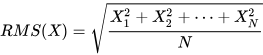
For stream processing, the time-series engine can calculate the RMS for each device using a one-second window that advances every second.
// Create a time-series engine with a 1000 ms window and a 10 ms step to calculate the RMS of accel
rms_engine = createTimeSeriesAggregator(
              name="rms_engine1",
              windowSize=1000,
              step=10,
              metrics=<[rms(accel)]>,
              dummyTable=vibration_raw,
              outputTable=vibration_rms,
              timeColumn=`timestamp,
              keyColumn=`deviceID,
              useSystemTime = true
              )
// Subscribe to the raw stream table and send the data to the engine
subscribeTable(
              tableName="vibration_raw",
              actionName="calc_rms",
              offset=0,
              handler=append!{rms_engine},
              msgAsTable=true
              );
Design notes:
-
windowSize=100specifies a window length of 100 milliseconds; -
step=10triggers a calculation every 10 milliseconds; -
metricsuses the predefinedrms(accel)function to calculate the RMS value; -
useSystemTime = truespecifies that system time, in milliseconds, is used as the time reference instead of the timestamp column.
7.3 Create an Anomaly Detection Engine for Threshold Alerts
Set the vibration severity alert threshold to 1.0. The system must detect whether the RMS exceeds this threshold and output an alert record.
// Create an anomaly detection engine to monitor RMS values
alert_engine = createAnomalyDetectionEngine(name="rms_alert1",
                                             metrics=<[rms > 1.0]>,
                                             dummyTable=vibration_rms,
                                             outputTable=vibration_alerts,
                                             keyColumn=`deviceID,
                                             timeColumn=`timestamp
                                         )
// Subscribe to the RMS result stream table and send the data to the anomaly detection engine
subscribeTable(
    tableName="vibration_rms",
    actionName="check_alert",
    offset=0,
    handler=append!{alert_engine},
    msgAsTable=true
    )
7.4 Real-Time Monitoring in Grafana
DolphinDB provides a Grafana data source plugin that supports direct queries against stream tables. For more information about the Grafana plugin, see DolphinDB Datasource.
After configuring the data source, enter the following SQL in Grafana's Query panel to monitor changes in the RMS metric for deviceID_1 in real time:
select * from vibration_rms where deviceID='deviceID_1'7.5 Summary
This example covers the key stages of ingesting vibration data, calculating RMS values in real time, generating threshold alerts, and visualizing the results in Grafana. You can copy and run the code directly. In practical applications, you can adjust the configuration based on the number of devices, sampling frequency, window parameters, and alert thresholds.
8. Appendix
-
Data ingestion script: genData.dos
-
Kafka ingestion script: createKafka.dos