
TSBS-Based Performance Comparison in IoT Scenarios
This report presents comparative tests of DolphinDB, InfluxDB, and TimescaleDB based on the Time Series Benchmark Suite (TSBS) in IoT scenarios. The tests evaluate write performance, query performance, and disk usage across deployment scales ranging from 100 to 10 million devices.
DolphinDB delivered the best overall performance in these tests. Across all five test scenarios, DolphinDB maintained high write throughput and a high compression ratio. It also retained strong read/write performance and scalability as the number of devices increased. For queries, DolphinDB generally provided shorter response times, with particularly notable advantages in large-scale deployments (1 million to 10 million devices) and latest-value queries.
The overall results show that DolphinDB performs well in high-frequency data ingestion, real-time querying, and storage efficiency when processing large-scale IoT time-series data, making it better suited to IoT applications requiring massive device connectivity and real-time analytics.
1. Test Scenarios
This test used the basic IoT dataset to simulate operational data from a fictitious freight company's truck fleet and to support to related data storage and operational analysis. Queries in this scenario cover real-time status monitoring and analysis and can scale with the fleet size, that is, the number of trucks. The dataset includes not only diagnostic data and operational metrics transmitted in real time by each truck, but also truck metadata. Queries associate operational metrics with diagnostic information. To better reflect real-world production environments, the dataset also includes out-of-order data and simulates the batch backfilling of data generated while vehicles are offline and transmitted after they reconnect.
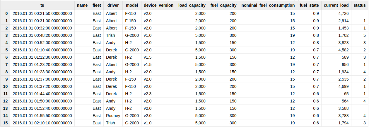
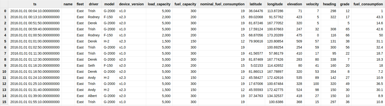
Each truck’s diagnostic data ("diagnostics") contains one nanosecond-precision timestamp, three measurements, and eight tag values. Each metrics record ("readings") contains one timestamp, seven measurements, and eight tag values. Examples of these data are shown in Figures 1-1 and 1-2.
The benchmark covers the following five scenarios. Table 1-1 summarizes the data volume and characteristics of each scenario.
| Scenario 1: 100 Devices | Scenario 2: 4,000 Devices | Scenario 3: 100,000 Devices | Scenario 4: 1,000,000 Devices | Scenario 5: 10,000,000 Devices | |
|---|---|---|---|---|---|
| Data interval | 10 seconds | 10 seconds | 10 seconds | 10 seconds | 10 seconds |
| Duration | 31 days | 4 days | 3 hours | 3 minutes | 3 minutes |
| Number of trucks | 100 | 4,000 | 100,000 | 1,000,000 | 10,000,000 |
| Records per truck | 241,145 | 31,118 | 972 | 16 | 16 |
| Number of records in the dataset | 48,229,186 | 248,944,316 | 194,487,997 | 32,414,619 | 324,145,090 |
2. Environment Configuration
To ensure a scientifically valid comparison, all three databases were tested on the same server under identical test environments, datasets, and scenarios.
2.1 Hardware and Software Configuration
The test server had the following hardware and software configuration:
-
Hardware Configuration
CPU: Intel(R) Xeon(R) Silver 4216 CPU @ 2.10 GHz
CPU cores: 64
Memory: 512 GB (16 × 32 GB DDR4 2400 MT/s)
Storage: one 3.2 TB solid-state drive (SSD)
-
Software Versions
DolphinDB Server V3.00.6.1
InfluxDB V1.8.10
TimescaleDB V2.10.1
Notes:
-
All databases were deployed in standalone mode.
-
InfluxDB V1.8.10, released in 2021, was selected because no TSBS-IOT implementation was publicly available for version 2.x.
2.2 Key Configuration Parameters
The following key parameters were configured for each evaluated database in the TSBS-IOT scenario to improve test performance.
-
DolphinDB
Enable the engine block cache.
setTSDBBlockCacheSize(50)-
InfluxDB
cache-max-memory-size = "80g"
index-version = "tsi1"
max-values-per-tag = 0
compact-full-write-cold-duration = "30s"-
TimescaleDB
CHUNK_TIME was configured differently for each scenario, as shown in the following table.
| Scenario 1 | Scenario 2 | Scenario 3 | Scenario 4 | Scenario 5 | |
|---|---|---|---|---|---|
| Number of trucks | 100 | 4,000 | 100,000 | 1,000,000 | 10,000,000 |
| Number of chunks | 12 | 12 | 12 | 12 | 12 |
| Chunk duration | 2.58 days | 8 hours | 15 minutes | 15 seconds | 15 seconds |
| CHUNK_TIME | 62 hours | 8 hours | 15 mimutes | 15 seconds | 15 seconds |
3. Test Conclusions
Based on test data, this study compared the write and query performance of DolphinDB, InfluxDB, and TimescaleDB in IoT applications. The overall results are as follows:
-
DolphinDB delivered the best overall performance. Across all five test scenarios, DolphinDB generally delivered the best performance in write throughput, write time, disk usage, and most query response times. As the number of devices increased from 100 to 10 million, DolphinDB maintained high write efficiency and relatively stable query performance, with its advantages becoming increasingly evident in large-scale device scenarios.
-
DolphinDB had a greater advantage at scale. In terms of write throughput, DolphinDB achieved approximately 1.9–10.7 times that of InfluxDB and 1.9–2.6 times that of TimescaleDB. In terms of disk usage, in scenarios involving 10 million devices, InfluxDB consumed approximately 96 times as much disk space as DolphinDB, while TimescaleDB consumed approximately 10.7 times as much. This indicates that as the number of devices and the data volume continue to grow, DolphinDB's advantages in write efficiency and storage cost become even more pronounced.
Write Performance Comparison:
-
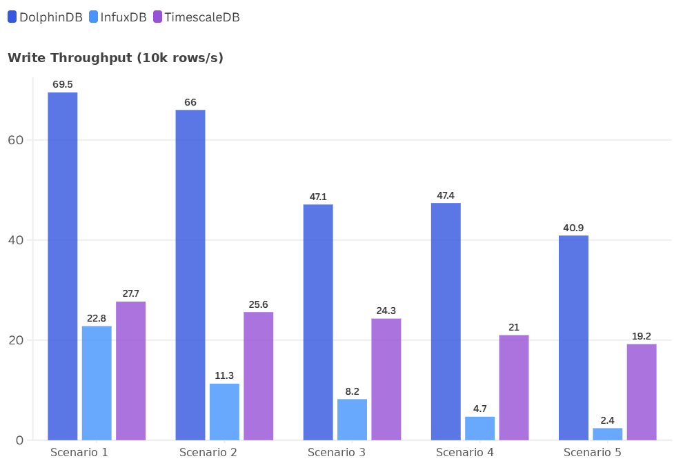
Highest write throughput. DolphinDB achieved write speeds of approximately 695K, 660K, 471K, 474K, and 409K rows per second in the five scenarios, respectively—higher than both InfluxDB and TimescaleDB in every scenario.
-
Shortest total write time. Across all five scenarios with identical data volumes, DolphinDB recorded the shortest total write time among the three databases, demonstrating superior ingestion efficiency.
-
Lower disk usage. DolphinDB used less disk space across all scenarios, with an especially significant advantage in large-scale scenarios. For example, in Scenario 5, DolphinDB used 5,355 MB of disk space, substantially less than InfluxDB's 515,990 MB and TimescaleDB's 57,426 MB.
-
More stable performance for large-scale writes. When the number of devices increased from 100 to 10 million, DolphinDB's write throughput declined somewhat but remained above 400,000 rows per second. This demonstrates its strong scalability and sustained write capability for large-scale IoT data ingestion.
Query Performance Comparison:
-
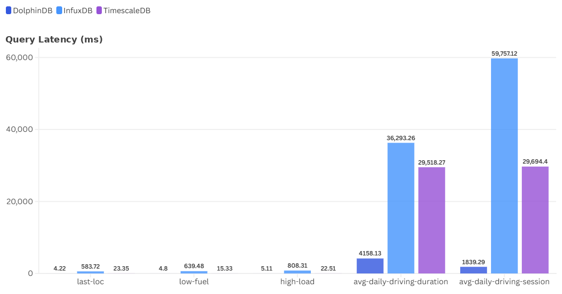
Shorter response times for small- and medium-sized device deployments. In Scenarios 1 and 2, DolphinDB maintained shorter average response times for all queries. Simple status queries were generally completed within milliseconds, and overall throughput was also higher. For example, in Scenario 2, InfluxDB's response times for most queries were approximately 2.6–187 times those of DolphinDB, while TimescaleDB's were approximately 3.2–29.3 times those of DolphinDB. As shown in Figure 3-2, DolphinDB had a clear advantage for both latest-value queries, such as last-loc, low-fuel, and high-load, and complex analytical queries, such as avg-daily-driving-duration and avg-daily-driving-session.
-
DolphinDB's advantage becomes more pronounced as the number of devices increases. In Scenarios 3 through 5, DolphinDB significantly outperformed InfluxDB and TimescaleDB on latest-value status queries. For example, for the last-loc query in Scenario 5, DolphinDB's average response time was 1,439.71 ms, compared with 234,950.25 ms for InfluxDB and 13,407.44 ms for TimescaleDB—approximately 163 times and 9.3 times longer than DolphinDB, respectively.
-
Overall, DolphinDB is better suited to large-scale IoT query and analytics workloads. It not only processes latest-value status queries faster but also provides stronger overall capabilities for complex analytical queries and massive data processing. It is better suited to high-volume time-series data applications such as connected vehicles, equipment monitoring, and industrial IoT.
4. Database Overview
DolphinDB's superior write performance is primarily attributable to its proprietary IoT engine, which is built upon the TSDB storage engine and tailored for the fine-grained, low-latency management of massive measurement points. The engine leverages a Log-Structured Merge-tree (LSM-tree) architecture—a hierarchical, ordered, disk-oriented data structure. By converting random writes into sequential writes, it significantly boosts write throughput to satisfy the demanding requirements of IoT applications. Compared to traditional B+ trees, LSM-trees inherently deliver superior write throughput. Building on this LSM-tree foundation, DolphinDB further optimizes write performance through efficient memory management, asynchronous writes, data compression, and other advanced techniques. Specifically, DolphinDB employs a PAX-based hybrid row-column storage layout and supports multiple compression algorithms, including LZ4, ZSTD, DELTA, and CHIMP. Compressing data columns on ingestion substantially reduces disk footprint and improves I/O efficiency. Furthermore, DolphinDB supports hash-based dimensionality reduction for index keys, preventing index metadata from growing excessively as device counts scale.
For queries, DolphinDB uses a storage architecture that combines partitioning, a primary index within each partition, and a secondary sparse index within each partition. This storage architecture is generally better suited to large-scale data workloads while also delivering good performance with smaller datasets. Its key advantages include:
-
PAX hybrid row-column storage: hybrid storage provides balanced query performance.
-
Hash-based dimensionality reduction (sortKeyMapping): This technology maps multiple indexes to suitable index ranges using a hash function, substantially reducing the indexing cost of massive numbers of time series and effectively addressing the most challenging problem in time-series databases: high cardinality, or an excessive number of time series.
-
Latest-value query optimization: For latest-value queries, the system can first read results from a latest-value cache table maintained by partition, avoiding scans of historical data.
InfluxDB uses its proprietary TSM storage engine, and its TSI time-series index is also based on an LSM-tree. InfluxDB 1.x organizes data by time series (series). A series is typically identified by a measurement, tag set, and field key. This approach has distinct advantages and disadvantages at different device scales. Its advantages include:
-
In small-scale device scenarios, the number of devices and tag combinations is relatively low, so the number of series is limited and the measurement/tag index structure is relatively simple, enabling rapid retrieval of the relevant time series.
-
With small data volumes, hot indexes and data are more likely to remain in the memory cache, reducing disk I/O during queries.
Its disadvantages include:
-
As the number of devices increases, the number of tag combinations grows, causing the number of time series (series cardinality) that InfluxDB must maintain to rise rapidly. As a result, queries must scan more index entries, which severely degrades query performance.
-
As the index structure expands, it consumes a large amount of memory at runtime, increasing the risk of out-of-memory conditions and affecting system stability.
-
When writing data from a large number of devices, InfluxDB must frequently update and maintain new series and their index information, causing its write performance to fall significantly behind.
-
With a large number of devices, the indexes and data can exceed available memory, resulting in more disk I/O operations and further degrading performance.
TimescaleDB is built on PostgreSQL and adds time-series optimizations. It divides time-series data along the time dimension into data blocks called chunks and applies indexes to each chunk to improve query performance. It has certain advantages for small-scale data workloads because of PostgreSQL's mature relational database functionality and flexible query capabilities. However, in large-scale, high-cardinality device-data scenarios, query and write performance are significantly constrained because the underlying architecture still relies on PostgreSQL's heap-based row storage and B-Tree indexes. When many devices write concurrently, data is distributed across time-based chunks, but indexes must still be continuously maintained within each active chunk. As the number of devices increases, the B-Tree index on "tags_id" and "time" must maintain index regions for more devices simultaneously. Because data from different devices is written to different index leaf pages, writes are no longer concentrated on a small number of hot pages. Instead, they switch among a large number of active leaf pages. If the number of active index pages exceeds the range that the in-memory cache can effectively retain, index-page reuse decreases, increasing the overhead of accessing disk pages. B-Tree insertions must also maintain index entries in order. When the target leaf page does not have enough free space, the index page may split. A large number of scattered inserts also increases random writes, ultimately causing write amplification. Each additional index requires the corresponding B-Tree to be updated during writes, further increasing disk I/O. Overall, this approach provides poor I/O efficiency when writing large volumes of time-series data.
5. Write Performance Comparison
5.1 Write Performance Comparison Across Scenarios
DolphinDB delivered higher write throughput and lower storage usage in all five test scenarios, with its advantages becoming more pronounced as the number of devices increased.
Across scenarios of different sizes, all three databases completed the writes in the 100-device and 4,000-device scenarios. However, DolphinDB completed the writes faster and achieved higher throughput. In the 100,000-device, 1-million-device, and 10-million-device scenarios, the data volume and number of devices increased substantially. InfluxDB and TimescaleDB experienced more pronounced declines in write throughput, while DolphinDB maintained throughput above 400,000 rows/s, demonstrating greater stability for large-scale writes.
In terms of disk usage, DolphinDB consumed less storage in every scenario, with the advantage becoming more pronounced at larger scales. For example, in Scenario 5, DolphinDB used 5,355 MB of disk space, significantly less than InfluxDB's 515,990 MB and TimescaleDB's 57,426 MB. This shows that DolphinDB can maintain effective data compression and storage efficiency while supporting high-frequency writes, making it suitable for continuous ingestion of large-scale IoT data.
Detailed test data is provided in the following tables:
| Scenario | Database | Row/s | Metrics/s | Elapsed Time (s) | Disk Usage (MB) |
|---|---|---|---|---|---|
| Scenario 1 | DolphinDB | 694,649.91 | 3,473,344.09 | 69.429 | 732 |
| InfluxDB | 228,465.05 | 1,806,412.25 | 211.101 | 814 | |
| TimescaleDB | 277,029.85 | 1,385,186.94 | 174.094 | 9,381 | |
| Scenario 2 | DolphinDB | 659,963.74 | 3,299,776.69 | 377.209 | 4,001 |
| InfluxDB | 112,619.06 | 890,426.78 | 2,210.499 | 4,255 | |
| TimescaleDB | 256,418.58 | 1,282,076.60 | 970.851 | 44,472 | |
| Scenario 3 | DolphinDB | 471,030.21 | 2,355,129.73 | 412.899 | 2,745 |
| InfluxDB | 81,808.29 | 646,821.95 | 2,377.363 | 4,068 | |
| TimescaleDB | 242,931.30 | 1,214,645.51 | 800.588 | 33,709 | |
| Scenario 4 | DolphinDB | 474,296.32 | 2,371,456.42 | 68.343 | 468 |
| InfluxDB | 47,459.47 | 375,244.93 | 682.996 | 3,706 | |
| TimescaleDB | 209,829.44 | 1,049,136.05 | 154.481 | 6,085 | |
| Scenario 5 | DolphinDB | 408,823.72 | 2,044,103.04 | 792.873 | 5,355 |
| InfluxDB | 24,243.77 | 191,685.36 | 13,370.245 | 515,990 | |
| TimescaleDB | 191,746.56 | 958,725.50 | 1,690.487 | 57,426 |
| DolphinDB/InfluxDB | DolphinDB/TimescaleDB | |
|---|---|---|
| 100 devices | 1.92x | 2.51x |
| 4,000 devices | 3.71x | 2.57x |
| 100,000 devices | 3.64x | 1.94x |
| 1,000,000 devices | 6.32x | 2.26x |
| 10,000,000 devices | 10.66x | 2.13x |
| InfluxDB/DolphinDB | TimescaleDB/DolphinDB | |
|---|---|---|
| 100 devices | 1.11x | 12.80x |
| 4,000 devices | 1.06x | 11.12x |
| 100,000 devices | 1.48x | 12.28x |
| 1,000,000 devices | 7.92x | 13.01x |
| 10,000,000 devices | 96.35x | 10.72x |
5.2 Resource Consumption During Writes
As shown in Table 5-4, DolphinDB's overall resource consumption during writes was low. The average CPU usage in Scenarios 3, 4, and 5 was 253%, 134%, and 295%, respectively. With one core equivalent to 100%, this corresponds to an actual average usage of approximately 1.3 to 3 CPU cores. Average memory usage was 11.70 GB, 7.95 GB, and 19.85 GB, respectively—a relatively small proportion of the test server's 512 GB of memory. Average disk write I/O remained between 37.69 MB/s and 44.79 MB/s. Write speed was limited by the TSBS setting of Workers=4 for concurrent writes. Increasing the number of concurrent writers could substantially improve DolphinDB's write speed.
Combined with the write performance results presented earlier, DolphinDB maintained a write throughput of approximately 400,000 to 470,000 rows/s in Scenarios 3 through 5. This shows that DolphinDB can sustain high write throughput while keeping CPU, memory, and disk I/O overhead relatively low in high-concurrency, large-scale IoT data ingestion scenarios. Overall, no obvious bottleneck in any single resource was observed during the write process, demonstrating good resource utilization efficiency and sustained write performance.
| Scenario | Average CPU Usage (1 core = 100%) | Average Memory Usage (GB) | Average Disk Write I/O (MB/s) |
|---|---|---|---|
| Scenario 3 | 253% | 11.70 | 40.00 |
| Scenario 4 | 134% | 7.95 | 37.69 |
| Scenario 5 | 295% | 19.85 | 44.79 |
6. Query Performance Comparison
Each test was executed with a concurrency of 4 worker threads, with each query repeated 100 times. Among the five test scenarios, Scenarios 1 and 2 each contained 12 query items, Scenario 3 contained 4, and Scenarios 4 and 5 each contained 3, for a total of 34 query items. The performance of each database is summarized below:
-
DolphinDB ranked first in 30 query items and second in the remaining 4.
-
InfluxDB ranked first in 1 query item, second in 7, and third in 26.
-
TimescaleDB ranked first in 3 query items, second in 23, and third in 8.
6.1 Query Performance in Scenario 1
In the small-scale device scenario represented by Scenario 1, DolphinDB delivered shorter average response times and higher query throughput for most query items. Its performance was particularly stable for the analytical queries long-driving-sessions, long-daily-sessions, avg-load, and breakdown-frequency. Overall, DolphinDB not only supports simple status queries effectively but also maintains low latency for complex grouped aggregations and time-window analysis, delivering the best overall query performance.
For long-daily-sessions, for example, DolphinDB delivered approximately 4–16 times the query performance of InfluxDB and TimescaleDB. The corresponding SQL statement is shown below.
select name, driver
from (
    select iif(avg(velocity) > 1, 1, 0) as driving
    from readings
    where readings.ts >= 2016.01.06T21:22:42.354897
    and readings.ts < 2016.01.07T21:22:42.354897
    and name is not null and fleet = "West"
    group by bar(ts, 10m), name, driver
)
group by name, driver
having sum(driving) > 60
This query is primarily used to count the periods during which vehicles continue driving over relatively long time ranges. The query consists of two layers. The inner query first aggregates data into 10-minute intervals by bar(ts,10m), name, driver, determining whether each vehicle was driving during each interval. The outer query then groups the results by name and driver, counts the intervals identified as driving periods, and filters for vehicle-driver combinations whose count exceeds the threshold.
Performance Advantages:
-
Because the query partitions data by day based on "ts", it can perform effective partition pruning, accessing only the partitions for the relevant dates and avoiding a full table scan.
-
"fleet" is an index key. For the filter condition fleet="West", the DolphinDB TSDB engine can use index information to exclude data blocks that do not contain the target data in advance, thereby reducing the amount of data that must actually be read. In the execution plan, this optimization appears as "TSDBIndexPrefiltering", which performs data-block prefiltering based on the TSDB index.
-
When creating a table within a TSDB database, "name", "fleet", and "ts" are specified as sort columns. After the data is written, it is sorted by vehicle name, fleet, and time. As a result, data for the same vehicle is relatively concentrated in physical storage and ordered chronologically. This storage layout facilitates grouping by name and driver and performing 10-minute interval aggregations. It reduces data reshuffling and intermediate computation during grouping, thereby improving aggregation efficiency.
| Query Item | Database | Mean Latency (ms) | Max Latency (ms) | Throughput (queries/s) |
|---|---|---|---|---|
| last-loc | DolphinDB | 5.40 | 7.63 | 710.56 |
| InfluxDB | 46.16 | 100.10 | 84.36 | |
| TimescaleDB | 1.92 | 27.02 | 1,830.21 | |
| low-fuel | DolphinDB | 5.55 | 8.34 | 696.85 |
| InfluxDB | 75.07 | 156.87 | 51.95 | |
| TimescaleDB | 2.05 | 39.49 | 1,711.37 | |
| high-load | DolphinDB | 6.25 | 11.50 | 610.34 |
| InfluxDB | 64.20 | 130.63 | 61.09 | |
| TimescaleDB | 2.18 | 37.84 | 1,475.11 | |
| stationary-trucks | DolphinDB | 4.70 | 17.39 | 804.71 |
| InfluxDB | 133.51 | 174.18 | 29.26 | |
| TimescaleDB | 4.88 | 25.25 | 739.41 | |
| long-driving-sessions | DolphinDB | 6.43 | 13.12 | 592.65 |
| InfluxDB | 25.69 | 70.85 | 152.54 | |
| TimescaleDB | 68.46 | 91.14 | 57.83 | |
| long-daily-sessions | DolphinDB | 14.11 | 26.55 | 270.88 |
| InfluxDB | 52.23 | 99.14 | 75.11 | |
| TimescaleDB | 232.38 | 447.21 | 16.75 | |
| avg-vs-projected-fuel-consumption | DolphinDB | 660.30 | 1062.21 | 6.02 |
| InfluxDB | 2,393.86 | 4,326.65 | 1.66 | |
| TimescaleDB | 8,564.34 | 21,685.25 | 0.46 | |
| avg-daily-driving-duration | DolphinDB | 750.10 | 1,320.51 | 5.25 |
| InfluxDB | 6,317.81 | 6,932.99 | 0.63 | |
| TimescaleDB | 5,143.83 | 11,326.46 | 0.75 | |
| avg-daily-driving-session | DolphinDB | 349.65 | 577.76 | 11.26 |
| InfluxDB | 9,372.36 | 9,896.45 | 0.43 | |
| TimescaleDB | 5,071.28 | 11,159.55 | 0.77 | |
| avg-load | DolphinDB | 466.79 | 765.95 | 8.52 |
| InfluxDB | 115,933.35 | 119,103.49 | 0.03 | |
| TimescaleDB | 2,745.15 | 6,471.68 | 1.44 | |
| daily-activity | DolphinDB | 1,176.14 | 1,771.07 | 3.36 |
| InfluxDB | 2,759.61 | 3,001.47 | 1.45 | |
| TimescaleDB | 5,365.12 | 11,704.32 | 0.74 | |
| breakdown-frequency | DolphinDB | 457.97 | 775.77 | 8.62 |
| InfluxDB | 54,796.96 | 56,346.62 | 0.07 | |
| TimescaleDB | 5,108.91 | 10,604.03 | 0.76 |
| Query Item | InfluxDB/DolphinDB | TimescaleDB/DolphinDB |
|---|---|---|
| last-loc | 8.55x | 0.36x |
| low-fuel | 13.53x | 0.37x |
| high-load | 10.27x | 0.35x |
| stationary-trucks | 28.41x | 1.04x |
| long-driving-sessions | 4.00x | 10.65x |
| long-daily-sessions | 3.70x | 16.47x |
| avg-vs-projected-fuel-consumption | 3.63x | 12.97x |
| avg-daily-driving-duration | 8.42x | 6.86x |
| avg-daily-driving-session | 26.81x | 14.50x |
| avg-load | 248.36x | 5.88x |
| daily-activity | 2.35x | 4.56x |
| breakdown-frequency | 119.65x | 11.16x |
6.2 Query Performance in Scenario 2
In Scenario 2, the number of devices increased. As the device count and data volume grew, query execution times increased for all three databases, but DolphinDB continued to deliver strong query performance. For latest-value queries and complex analytical queries, DolphinDB outperformed InfluxDB and TimescaleDB in most cases. In particular, for latest-status queries such as last-loc, low-fuel, and high-load, DolphinDB consistently maintained low query latency. It also demonstrated clear advantages in complex queries such as avg-daily-driving-session, avg-load, and breakdown-frequency.
6.2.1 Analysis of Latest-Value Queries
The following SQL statement is used to analyze SQL optimization for last-loc.
select * from (
    select name, driver, longitude, latitude
    from readings
    where fleet = "South"
    context by name, fleet csort ts limit -1)
where name is not null
This query retrieves the latest location and driver information for each truck in a fleet. The query first selects the vehicle data in the "readings" sensor data table to retain vehicles where fleet="South". It then groups the data by name and fleet—that is, by vehicle and fleet. Within each group, records are sorted by the "ts" time column, and limit-1 retrieves the last record in each group, representing the vehicle's latest record.
Performance Advantages:
-
When querying latest values with the
context by [id, tag] csort [ts] limit -1clause, the WHERE filter includes the firstSortKey column (fleet) with the equality operator (=). This satisfies the prerequisites for the latest-value cache table, enabling DolphinDB to fetch results directly from memory and eliminate disk I/O.
6.2.2 Complex Mixed Queries
The following SQL statement is used to analyze SQL optimization for avg-daily-driving-session.
select
    name,
    day,
    driving_buckets * 600000.0 / session_count as avg_duration
from (
    select
        sum(is_driving) as driving_buckets,
        sum(driving_change == 1) + first(is_driving) as session_count
    from (
        select
            name,
            date(bar_ts) as day,
            bar_ts,
            is_driving,
            deltas(is_driving) as driving_change
        from (
            select avg(velocity) > 5 as is_driving
            from readings
            where ts >= 2016.01.01T00:00:00.000
              and ts < 2016.01.05T00:00:00.000
              and name is not null
            group by name, bar(ts, 10m) as bar_ts
        )
        context by name, date(bar_ts)
        csort bar_ts
    )
    group by name, day
)
where session_count > 0
This query calculates each driver's average continuous driving duration per day. It first aggregates the raw data into 10-minute windows for each driver and determines whether the driver was driving during each window based on the average speed. It then sorts the driving states by driver and date and identifies changes in state to determine the number of driving sessions per day. Finally, it calculates the total driving duration from the number of 10-minute windows during which the driver was driving that day, then divides it by the number of driving sessions to obtain each driver's average continuous driving duration per day.
Performance Advantages:
-
The "readings" table is partitioned by "name" and "ts". The query can use "ts" to perform effective daily partition pruning, accessing only the partitions for the relevant dates and avoiding a full table scan.
-
The "readings" table is sorted by "name", "fleet", and "ts". The inner aggregation in this query takes advantage of the TSDB table's ordered storage, reducing the overhead of grouped aggregation.
| Query Item | Database | Mean Latency (ms) | Max Latency (ms) | Throughput (queries/s) |
|---|---|---|---|---|
| last-loc | DolphinDB | 4.22 | 8.18 | 898.31 |
| InfluxDB | 583.72 | 735.87 | 6.81 | |
| TimescaleDB | 23.35 | 239.31 | 164.10 | |
| low-fuel | DolphinDB | 4.80 | 8.03 | 798.37 |
| InfluxDB | 639.48 | 796.93 | 6.23 | |
| TimescaleDB | 15.33 | 57.04 | 252.93 | |
| high-load | DolphinDB | 5.11 | 8.81 | 734.77 |
| InfluxDB | 808.31 | 961.92 | 4.90 | |
| TimescaleDB | 22.51 | 230.20 | 172.29 | |
| stationary-trucks | DolphinDB | 42.75 | 73.00 | 91.20 |
| InfluxDB | 2,485.77 | 3,046.66 | 1.57 | |
| TimescaleDB | 138.56 | 280.16 | 28.53 | |
| long-driving-sessions | DolphinDB | 75.70 | 106.92 | 51.61 |
| InfluxDB | 282.38 | 408.30 | 14.00 | |
| TimescaleDB | 1,754.84 | 3,559.30 | 2.20 | |
| long-daily-sessions | DolphinDB | 287.18 | 654.69 | 13.67 |
| InfluxDB | 1,044.11 | 1,288.51 | 3.81 | |
| TimescaleDB | 8,412.73 | 18,275.33 | 0.47 | |
| avg-vs-projected-fuel-consumption | DolphinDB | 4,508.60 | 7,436.80 | 0.88 |
| InfluxDB | 11,655.38 | 15,793.15 | 0.34 | |
| TimescaleDB | 30,206.93 | 69,693.44 | 0.13 | |
| avg-daily-driving-duration | DolphinDB | 4,158.13 | 6,989.57 | 0.95 |
| InfluxDB | 36,293.26 | 38,184.96 | 0.11 | |
| TimescaleDB | 29,518.27 | 66,535.42 | 0.13 | |
| avg-daily-driving-session | DolphinDB | 1,839.29 | 3,141.12 | 2.15 |
| InfluxDB | 59,757.12 | 62,808.06 | 0.07 | |
| TimescaleDB | 29,694.40 | 65,882.11 | 0.13 | |
| avg-load | DolphinDB | 2,697.22 | 5,038.59 | 1.46 |
| InfluxDB | 504,725.18 | 515,162.11 | 0.01 | |
| TimescaleDB | 17,887.90 | 37,890.05 | 0.22 | |
| daily-activity | DolphinDB | 6,537.10 | 11,950.59 | 0.61 |
| InfluxDB | 5,632.81 | 6,403.07 | 0.71 | |
| TimescaleDB | 32,822.26 | 95,600.64 | 0.12 | |
| breakdown-frequency | DolphinDB | 2,633.96 | 4,814.59 | 1.51 |
| InfluxDB | 299,388.11 | 305,856.51 | 0.01 | |
| TimescaleDB | 30,038.50 | 63,655.93 | 0.13 |
| Query Item | InfluxDB/DolphinDB | TimescaleDB/DolphinDB |
|---|---|---|
| last-loc | 138.32x | 5.53x |
| low-fuel | 133.23x | 3.19x |
| high-load | 158.18x | 4.41x |
| stationary-trucks | 58.15x | 3.24x |
| long-driving-sessions | 3.73x | 23.18x |
| long-daily-sessions | 3.64x | 29.29x |
| avg-vs-projected-fuel-consumption | 2.59x | 6.70x |
| avg-daily-driving-duration | 8.73x | 7.10x |
| avg-daily-driving-session | 32.49x | 16.14x |
| avg-load | 187.13x | 6.63x |
| daily-activity | 0.86x | 5.02x |
| breakdown-frequency | 113.66x | 11.40x |
6.3 Query Performance in Scenario 3
In Scenario 3, the device count increased further to 100,000. This scenario included four query items: last-loc, low-fuel, high-load, and stationary-trucks. The test results showed that DolphinDB had a significantly lower average response time than InfluxDB and TimescaleDB for every query item. Even with the substantial increase in device count, DolphinDB continued to effectively control the execution overhead of latest-status and device-filtering queries, demonstrating better scalability for querying large numbers of devices.
| Query Item | Database | Mean Latency (ms) | Max Latency (ms) | Throughput (queries/s) |
|---|---|---|---|---|
| last-loc | DolphinDB | 66.54 | 451.45 | 59.17 |
| InfluxDB | 6,381.56 | 7,876.10 | 0.62 | |
| TimescaleDB | 225.52 | 422.33 | 17.58 | |
| low-fuel | DolphinDB | 45.37 | 67.42 | 85.41 |
| InfluxDB | 9,576.72 | 11,016.70 | 0.42 | |
| TimescaleDB | 214.55 | 365.73 | 18.28 | |
| high-load | DolphinDB | 71.87 | 450.13 | 54.44 |
| InfluxDB | 8,770.11 | 10,824.70 | 0.45 | |
| TimescaleDB | 214.19 | 401.36 | 18.57 | |
| stationary-trucks | DolphinDB | 201.59 | 559.29 | 19.39 |
| InfluxDB | 45,761.18 | 55,879.68 | 0.09 | |
| TimescaleDB | 1,316.01 | 3,090.69 | 2.97 |
Note: In Scenario 3, TSBS only generates queries for last-loc, low-fuel, high-load, and stationary-trucks.
6.4 Query Performance in Scenario 4
With 1 million devices in Scenario 4, InfluxDB and TimescaleDB had significantly longer response times than DolphinDB, and the performance gap widened further. For latest-status queries, DolphinDB's average response time remained in the hundreds of milliseconds, while InfluxDB's increased to several seconds or even tens of seconds. TimescaleDB also exhibited significantly higher response times than DolphinDB. This demonstrated that DolphinDB can effectively support high-cardinality device state queries even at the million-device scale.
| Query Item | Database | Mean Latency (ms) | Max Latency (ms) | Throughput (queries/s) |
|---|---|---|---|---|
| last-loc | DolphinDB | 128.97 | 175.98 | 30.05 |
| InfluxDB | 18,470.30 | 20,192.26 | 0.22 | |
| TimescaleDB | 1,327.57 | 1,597.69 | 2.99 | |
| low-fuel | DolphinDB | 125.78 | 179.92 | 31.55 |
| InfluxDB | 12,514.69 | 14,065.66 | 0.32 | |
| TimescaleDB | 1,205.62 | 1,459.58 | 3.27 | |
| high-load | DolphinDB | 129.96 | 168.56 | 30.55 |
| InfluxDB | 28,789.58 | 30,387.20 | 0.14 | |
| TimescaleDB | 1,402.48 | 2,158.72 | 2.77 |
Note: In Scenario 4, TSBS only generates queries for last-loc, low-fuel, and high-load.
6.5 Query Performance in Scenario 5
With 10 million devices in Scenario 5, DolphinDB continued to significantly outperform InfluxDB and TimescaleDB in query performance. Although DolphinDB's response times increased compared with the preceding scenarios, they remained within the seconds range for latest-status queries. By contrast, InfluxDB's query execution times increased substantially, while TimescaleDB reached approximately the tens-of-seconds range. Overall, DolphinDB continued to provide good query availability and stability at the tens-of-millions device scale, making it better suited to high-cardinality, large-scale IoT device-status query scenarios.
| Query Item | Database | Mean Latency (ms) | Max Latency (ms) | Throughput (queries/s) |
|---|---|---|---|---|
| last-loc | DolphinDB | 1,439.71 | 1,756.10 | 2.77 |
| InfluxDB | 234,950.25 | 269,008.90 | 0.02 | |
| TimescaleDB | 13,407.44 | 16,209.41 | 0.30 | |
| low-fuel | DolphinDB | 1,346.10 | 1,625.34 | 2.95 |
| InfluxDB | 158,430.33 | 179,486.72 | 0.03 | |
| TimescaleDB | 12,540.57 | 14,479.36 | 0.32 | |
| high-load | DolphinDB | 1,451.00 | 1,854.78 | 2.74 |
| InfluxDB | 745,830.65 | 2,775,056.38 | 0.01 | |
| TimescaleDB | 13,286.57 | 15,211.52 | 0.29 |
Note: In Scenario 5, TSBS only generates queries for last-loc, low-fuel, and high-load.
6.6 Query Resource Consumption
Because some queries run for an extremely short time, the server's CPU, memory, and I/O usage cannot be observed throughout the entire query process. For Scenario 2, complex queries such as avg-daily-driving-duration were executed 100 times to record server CPU and memory utilization throughout the query execution process.
| Query Item | Average CPU Usage (1 core = 100%) | Average Memory Usage (GB) |
|---|---|---|
| avg-daily-driving-duration | 2,264% | 6.98 |
| avg-daily-driving-session | 2,305% | 6.19 |
| avg-load | 2,353% | 6.57 |
| daily-activity | 2,411% | 6.03 |
| breakdown-frequency | 2,409% | 7.59 |
The query resource utilization results show that DolphinDB primarily consumed CPU resources when executing complex analytical queries in Scenario 2. The average CPU utilization of queries such as avg-daily-driving-duration, avg-daily-driving-session, avg-load, daily-activity, and breakdown-frequency is generally high. With 100% representing one full CPU core, these queries utilized approximately 22 to 26 CPU cores on average, proving that DolphinDB effectively exploits multi-core parallel processing for complex aggregations and analytical workloads.
Memory consumption remained relatively stable across all queries, generally ranging from 6 to 8 GB. This represented a small proportion of the test server's total memory, with no significant memory pressure observed. This indicates that although these queries are computationally intensive, their memory usage remains manageable.
7. Test Summary
Based on the results of this TSBS IoT benchmark, DolphinDB is an excellent time-series database for IoT applications. In the standalone test environment, DolphinDB delivered strong performance in write throughput, query response time, and disk space utilization. Its high-throughput ingestion, efficient querying, and low storage costs make it well-suited to large-scale time-series data applications such as connected vehicles, equipment monitoring, and the Industrial IoT.
The test results in this report can also serve as a benchmark reference for selecting and evaluating time-series databases in IoT scenarios. They provide architects with a basis for system architecture design, capacity planning, and resource allocation in specific production applications. Note that these tests were conducted in a standalone environment. In production, DolphinDB can further scale write and query capabilities through cluster deployment. With appropriately designed data partitions and effective load balancing, overall throughput can increase linearly as cluster nodes are added.
Further Reading:
-
IoT Engine: How to use the IoT engine to optimize tag management, latest-value queries, and large-scale device data analysis. IOT Engine
-
Cluster Tutorial: How to deploy, scale, and configure high availability for a DolphinDB cluster. High-availability Cluster Deployment
-
Hot and Cold Data Tiering: How to balance low storage costs with high query performance. Tiered Storage
Attachments
Complete Test Files and Code: tsbs-dolphindb.zip. See docs/dolphindb.md in the test package for the test procedure.