
Implementing a Multi-Factor Risk Model in DolphinDB
Modern quantitative finance requires robust frameworks to navigate the complexities of large-scale equity markets. A prime example is the MSCI China A-Share Equity Model (CNE6). While specifically designed for the Chinese market, the CNE6 framework represents a sophisticated multi-layered factor architecture that addresses universal challenges in risk estimation: capturing precise cross-sectional exposures across diverse style factors while maintaining temporal memory.
This model is not just a regional tool; it serves as a scalable blueprint for any market requiring high-precision risk decomposition, portfolio optimization, and risk assessment. In this tutorial, we demonstrate how to leverage DolphinDB’s high-performance vectorized engine to implement this complex model—from handling massive cross-sectional regressions to performing advanced risk adjustments like Newey-West, Eigenfactor adjustment, and Bayesian Shrinkage.
Note: While this tutorial uses China A-share data and regional factor definitions (such as CNE6), the underlying Barra model architecture and DolphinDB implementation are market-agnostic. You can seamlessly adapt this workflow to global markets by substituting local risk factors and industry classifications while maintaining the same computational logic.
1. Introduction to the Multi-Factor Model
1.1 The Multi-Factor Model
The multi-factor model employs a factor regression framework to jointly model asset returns with style, market, and industry factors, estimating both factor returns and idiosyncratic returns. The multi-factor risk model constructed in this article follows the CNE6 model.
The CNE6 model is a multi-factor model designed for the Chinese stock market. This model incorporates one country factor, multiple industry factors, and multiple style factors. Assume there are N stocks, P industries, and Q style factors in the market. At any given point in time, the model uses factor exposures and individual stock returns to construct the following cross-sectional regression:

where:
-
rn is the return of stock n, and rf is the risk-free return.
-
XnIp is the exposure of stock n to industry Ip. Assuming a company belongs to only one industry, XnIp takes the value 0 (the stock does not belong to that industry) or 1 (the stock belongs to that industry).
-
XnIp is the exposure of stock n to style factor Sq, and its value has been standardized (the standardization method is explained below).
-
un is the portion of the excess return of stock n that cannot be explained by the factors, and is therefore also known as the stock's idiosyncratic return.
-
fC is the factor return of the country factor (all stocks have an exposure of 1 to the country factor).
-
fIp is the factor return of industry factor Ip.
-
fSq is the factor return of style factor Sq.
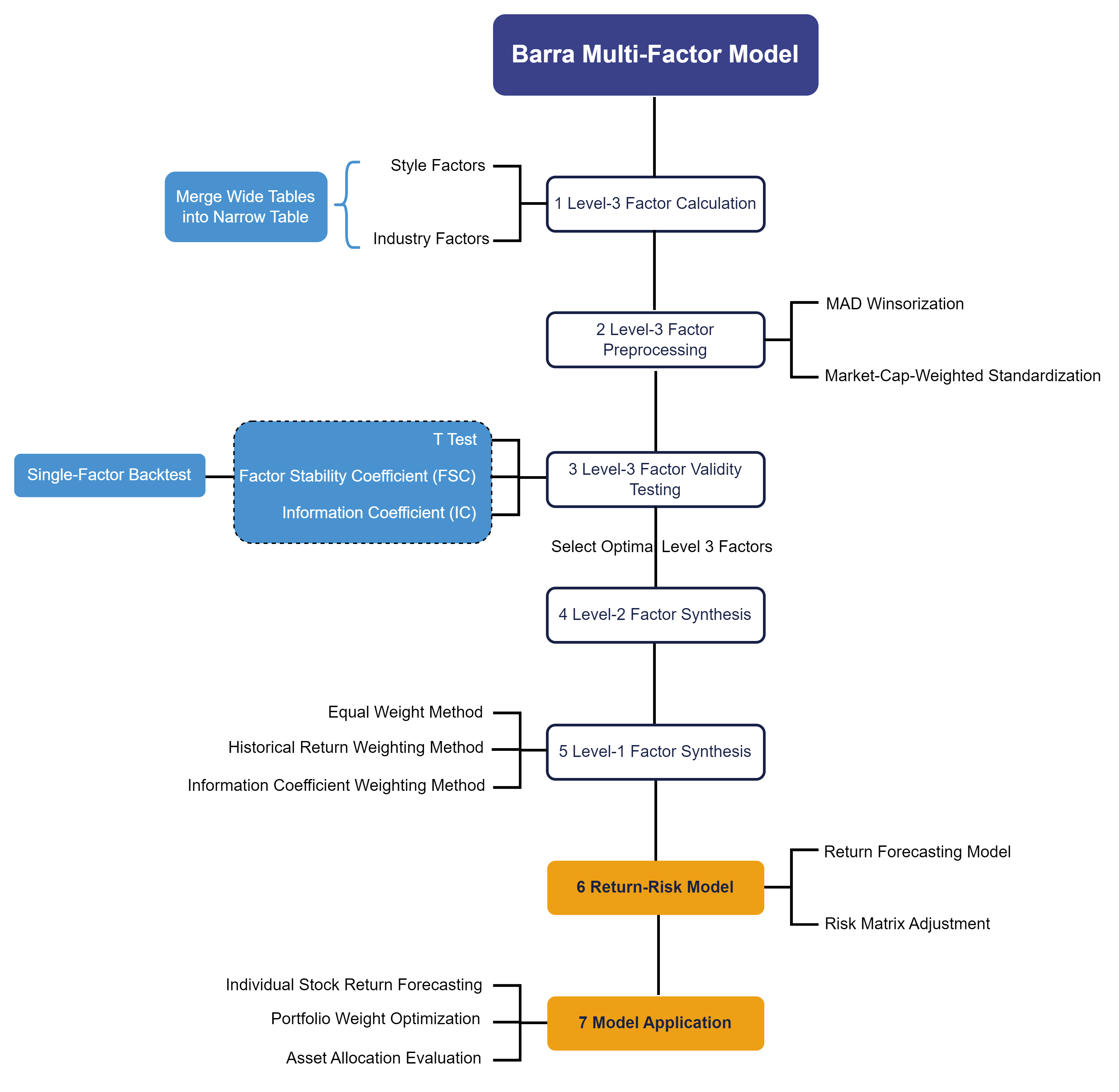
The following figure shows the workflow of the multi-factor model. The workflow starts with the computation of raw factors, followed by single-factor evaluation to assess each candidate factor in terms of stability, predictive power, and consistency. Based on the evaluation results, DolphinDB APIs are used to construct the required Level-1 and Level-2 factors. For the synthesized factors, DolphinDB builds a return forecasting model and adjusts the risk matrix, then evaluates the model in terms of goodness of fit, bias statistics, and Q statistics. Finally, the return-risk model is used for portfolio risk assessment and portfolio optimization.
1.2 Return-Risk Model
The core objective of a multi-factor model is to quantify the risks of individual stocks and factors, and to support investment decisions via time-series analysis of returns and risks. The CNE6 model expresses an individual stock's return as a linear combination of factor returns and its idiosyncratic return.
where r is the N*1 vector of individual stock returns, X is the current factor exposure matrix (N*k, where k is the number of factors), f is the k*1 vector of factor returns, and u is the N*1 vector of idiosyncratic returns. The formula is r=Xf+u.
Taking the covariance matrix on both sides of the above equation yields the following formula, which decomposes the stock covariance matrix V into the factor return covariance matrix Vf and the idiosyncratic return covariance matrix Δ. The formula is V=XVfX'+Δ.
When risk is assessed from the stock return covariance matrix, the matrix may be rank-deficient because the number of stocks N is far greater than the number of trading days (252), and it would require N*(N+1)/2 calculations, which is extremely complex. With the multi-factor risk model, obtaining the stock return risk matrix V only requires the factor return risk matrix Vf and the idiosyncratic return risk matrix Δ, requiring only n*(n+1)/2+N calculations. This further avoids the rank-deficiency problem of the return covariance matrix.
2. Factor Synthesis Using DolphinDB
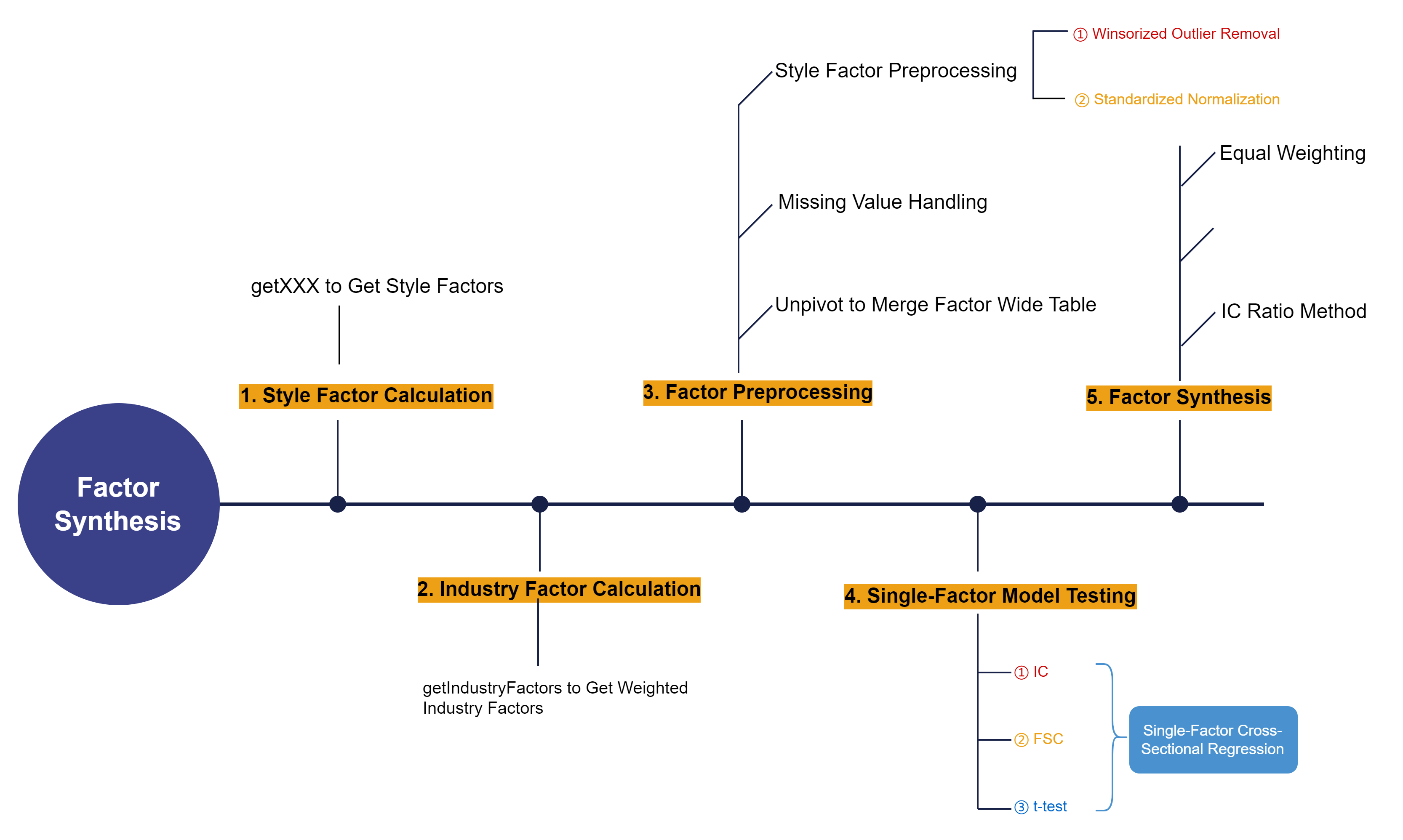
This article first uses the RiskFactorsCal module to obtain the multi-factor narrow table for modeling. The detailed process is as follows:
-
Calculate style factors using the
getXXXXfunction. -
Calculate industry factors using the
getIndustryFactorsfunction. -
Use the
getRegTablefunction to merge style and industry factors and fill missing values, producing a regression factor table for single-factor model validation. -
Use the
getFactorsValidationfunction to generate the IC and metrics for each factor in the regression factor table. -
For different factor weighting methods, use the
getFSLevelFactorfunction to synthesize Level-3 factors into the Level-1 factor narrow table for building the multi-factor model.
2.1 Style Factor Caculation
First, individual Level-3 style factors are calculated. Level-1 and Level-2 style factors are then synthesized based on the style factor relationship table below. Among them, predictive factors such as ETOPF_STD, ETOPF, EGRLF, and DTOPF have unstable effects on the model and are excluded for now.
Table 2-1 Style Factor Mapping
| Level-1 Factor | Level-2 Factor | Level-3 Factor | Definition | Level-3 Factor Function | Level-3 Factor Input Parameters |
|---|---|---|---|---|---|
| Quality | Earnings Quality | ABS | Balance sheet accruals | getAbs |
|
| ACF_TTM | Cash flow statement accruals (rolling) | getAcf |
method='TTM' |
||
| ACF_LYR | Cash flow statement accruals (static) | getAcf |
method='LYR' |
||
| Earnings Variability | VSAL_TTM | Revenue volatility (rolling) | getVsal |
method='TTM' |
|
| VSAL_LYR | Revenue volatility (static) | getVsal |
method='LYR' |
||
| VERN_TTM | Earnings volatility (rolling) | getVern |
method='TTM' |
||
| VERN_LYR | Earnings volatility (static) | getVern |
method='LYR' |
||
| VFLO_TTM | Cash flow volatility (rolling) | getVflo |
method='TTM' |
||
| VFLO_LYR | Cash flow volatility (static) | getVflo |
method='LYR' |
||
| Investment Quality | AGRO | Total asset growth rate | getAgro |
||
| IGRO | New share issuance growth rate | getIgro |
|||
| CXGRO | Capital expenditure growth rate | getCxgro |
|||
| Leverage | MLEV | Market leverage | getMlev |
||
| BLEV | Book leverage | getBlev |
|||
| DTOA | Asset-liability ratio | getDtoa |
|||
| Profitability | ATO_TTM | Asset turnover (rolling) | getAto |
method='TTM' |
|
| ATO_LYR | Asset turnover (static) | getAto |
method='LYR' |
||
| GP_TTM | Asset gross margin (rolling) | getGp |
method='TTM' |
||
| GP_LYR | Asset gross margin (static) | getGp |
method='LYR' |
||
| GPM_TTM | Sales gross margin (rolling) | getGpm |
method='TTM' |
||
| GPM_LYR | Sales gross margin (static) | getGpm |
method='LYR' |
||
| ROA_TTM | Return on total assets (rolling) | getRoa |
method='TTM' |
||
| ROA_LYR | Return on total assets (static) | getRoa |
method='LYR' |
||
| Value | Btop | BTOP | Book-to-market ratio | getBtop |
|
| Earning Yield | CETOP_TTM | Cash earnings yield (rolling) | getCetop |
method='TTM' |
|
| CETOP_LYR | Cash earnings yield (static) | getCetop |
method='LYR' |
||
| ETOP_TTM | Forecast earnings yield (rolling) | getEtop |
method='TTM' |
||
| ETOP_LYR | Forecast earnings yield (static) | getEtop |
method='LYR' |
||
| EM | Earnings-to-enterprise value ratio | getEm |
|||
| Long-Term Reversal | LTRSTR | Long-term reversal relative strength | getLtrstr |
||
| LTHALPHA | Long-term reversal excess returns | getLthalpha |
|||
| Growth | Growth | EGRO_TTM | Revenue per share growth (rolling) | getEgro |
method='TTM' |
| EGRO_LYR | Revenue per share growth (static) | getEgro |
method='LYR' |
||
| SGRO_TTM | Earnings per share growth (rolling) | getSgro |
method='TTM' |
||
| SGRO_LYR | Earnings per share growth (static) | getSgro |
method='LYR' |
||
| Liquidity | Liquidity | STOM | Monthly turnover rate | getStom |
|
| STOQ | Quarterly turnover rate | getStoq |
|||
| STOA | Annual turnover rate | getStoa |
|||
| ATVR | Annualized trading ratio | getAtvr |
|||
| Volatility | Beta | HBETA | Beta | getHbeta |
|
| Residual Volatility | HSIGMA | Idiosyncratic volatility | getHsigma |
||
| DASTD | Volatility | getDastd |
|||
| CMRA | Cumulative return | getCmra |
|||
| Size | Size | LNCAP | Log market cap | getLncap |
|
| Mid Cap | MIDCAP | Mid-cap | getMidcap |
||
| Momentum | Momentum | RSTR | Market relative strength | getRstr |
|
| HALPHA | Historical excess returns | getHalpha |
|||
| Dividend Yield | Dividend Yield | DTOP | Dividend yield | getDtop |
When calculating an individual Level-3 style factor, call the function get + the factor name. For example, the calculation of the Blev (Beta Leverage), Stom (Size Turnover Momentum), and Stoq (Stock Quality) factors is as follows:
getBlev(startTime = 2022.01.03,windows = 365,endTime = 2023.01.02)
getStom(startTime = 2022.01.03,windows = 21,endTime = 2023.01.02)
getStoq(startTime = 2022.01.03,windows = 63,endTime = 2023.01.02)
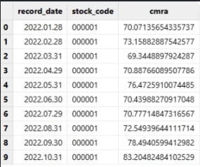
Each single-factor calculation function returns a narrow table. The results are roughly as follows:
2.2 Industry Factor Calculation
Industry dummy factors are constructed based on the Level-1 Shenwan (SW_2021) and CITIC industry classifications. CNLT assigns weights based on market capitalization, and the API provides market-capitalization-weighted industry factors.
Table 2-2 Industry Dummy Factors Calculation
| API | Description |
|---|---|
getIndustry |
Obtain the raw industry factor
|
getIndustryWeighted |
Obtain the industry factor weights
|
getIndustryFactor |
Obtain the weighted industry factors
|
Partial returned results are as follows:
getIndustry(startTime = 2022.01.01,endTime = 2023.01.02,method = 'SW_2021')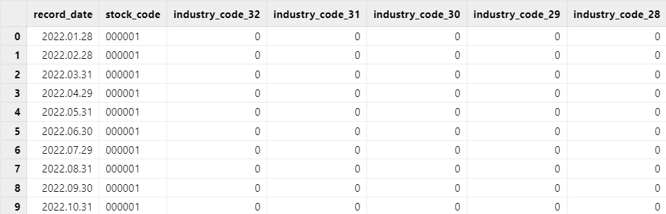
getIndustryWeighted(startTime = 2022.01.03,endTime = 2023.01.02,method = 'SW_2021')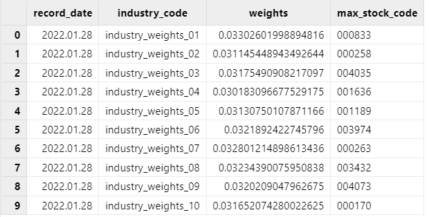
getIndustryFactor(startTime = 2022.01.03,endTime = 2023.01.02,method = 'SW_2021')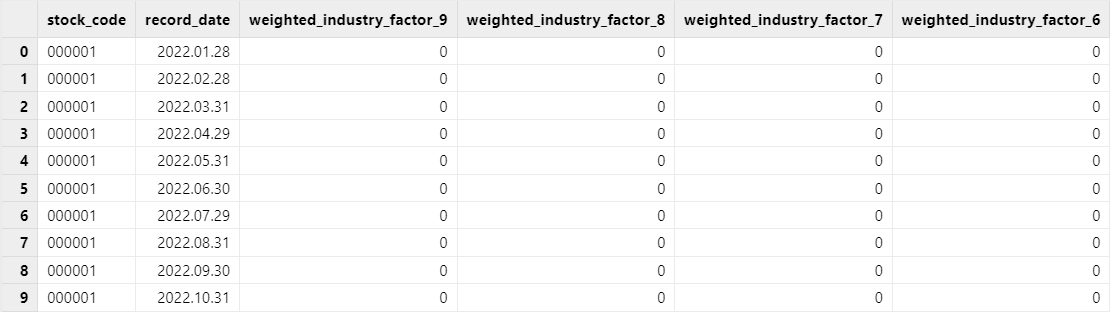
2.3 Factor Preprocessing
After the raw Level-3 style factors are calculated, a standardized data-cleaning pipeline is usually required before further factor synthesis. DolphinDB uses the MAD (median absolute deviation) method to winsorize extreme values and applies CNLT's market-capitalization standardization process.
2.3.1 MAD-Based Outlier Removal for Style Factors
The MAD method uses the median. Compared with the traditional mean-standard deviation method, it is robust and not affected by extreme outliers. It is an improvement over the approach that subtracts the mean and uses the standard deviation. The advantage of the MAD method over other outlier detection methods is its strong robustness to outliers. The function corresponding to the MAD method in this article is winsorized.
/* winsorized
Winsorize the factor table.
The factor table must contain three columns: record date, stock code, and raw factor, with the raw factor as the third column.
Input:
         tbName
Output:
         factor table after winsorized
*/
The MAD method is implemented as follows:
-
Calculate the median of the dataset as the measure of central tendency.
-
For each data point, calculate its absolute deviation from the median.
-
Calculate the median of all absolute deviations, i.e., the median absolute deviation (MAD).
MAD = median(|Xi -median(X)| )
-
Determine the threshold for identifying outliers. Typically, a data point is considered an outlier if its deviation from the median exceeds a specified multiple of the MAD, such as 3 times the MAD.
-
Identify outliers. Data points exceeding the threshold can be marked as outliers or subjected to further analysis.
2.3.2 Market-Cap-Weighted Standardization of Style Factors
Market-cap-weighted standardization is intended to remove the impact of extreme market capitalization on factor calculation contributions (CNLT). This method brings the factor scales to a comparable level. For the n-th stock and its k-th raw factor exposure , the standardization process is ,
where μk and σk are, respectively, the market-cap-weighted mean and the equal-weighted standard deviation of factor k.
The standardized function implements market-cap-weighted standardization. Set adjusted=true to apply market-cap neutralization.
/* standardized
Standardize and market-neutralize the factor table.
The factor table must contain three columns: record date, stock code, and raw factor, with the raw factor as the third column.
Input:
         tbName
         adjusted    Market-neutralize or not
Output:
         factor table after standardized
*/
2.3.3 Combine Style and Industry Factors
The two functions winsorized and standardized are integrated into the getAllFactors function. getAllFactors performs standardization and outlier removal through the parameters normlizing and scaling, respectively. In addition, after obtaining the industry and style factors, the getAllFactors function returns a wide table that combines all the above factors and can be further used for single-factor effectiveness testing.
/* getAllFactors
Get all factors.
Input:   normlizing: true (Default) Standardization
         scaling: true (Default) Outlier removal
         decap: true (Default) Market-neutralization
         industry_weighted: true (Default) Industry market-cap weighting
         industry_method: 'CITIC' (Default), 'SW_2021'
         startTime: 2022.01.03 (Default)
         endTime: 2023.01.02 (Default)
Output:
         factor table
*/
Factors = getAllFactors(st=st,et =et, normlizing = true,
scaling = true,decap = false,industry_method = 'CITIC',
industry_weighted = false)
select * from Factors limit 1002.3.4 Handle Missing Factor Values
Before building the factor regression model, missing factor values must be further processed to avoid their impact on the regression results. In this article, the function for handling missing values of all raw factors is getRegTable, and mean imputation is used to fill missing values.
/* getRegTable
Get a processed regression factor table for regression, including stock returns, factor exposures, industry factors, industry variables, and regression weights.
Input:
         factorsTable: false (Default) Whether to use the provided initial factor table
         tbName: NULL (Default) Initial factor table
         normlizing: true (Default) Standardization
         scaling: true (Default) Outlier removal
         decap: true (Default) Market-neutralization for regression
         industry_weighted: true (Default) Industry factor weighting
         industry_method: 'CITIC' (Default), 'SW_2021'
         st: 2022.01.03 (Default)
         et: 2023.01.02 (Default)
Output:
         regression table
*/
Note:
The initial factor table tbName is required only when factorsTable is true. In this case, you must pass a full factor table that has already been standardized, winsorized, market-neutralized, and industry-weighted using the getAllFactors function (or a partial factor table after filtering stocks). Consequently, the parameters normlizing, scaling, decap, and industry_weighted have no effect on the result whether they are false or true. That is, tmpReg = getRegTable(factorsTable = true,tbName = Factors,st= st,et = et).
fTable = getRegTable(factorsTable = true,tbName = Factors,st= st,
                     et = et,normlizing = normlizing ,scaling = scaling,
                     decap = decap, industry_method = industry_method,
                     industry_weighted = industry_weighted)
After running the command above, the comparison of data before and after processing is as follows:
Before processing, the raw Level-3 factor wide table generated by getAllFactors:
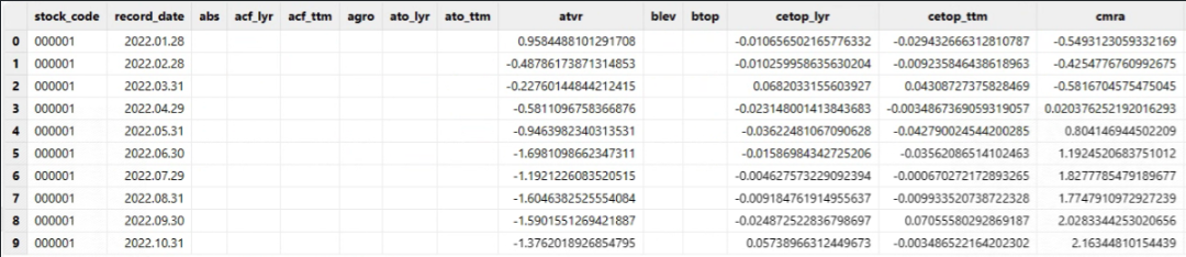
After processing, the Level-3 factor wide table cleaned (e.g., missing values filled) by getRegTable:

2.4. Single-Factor Model Testing
2.4.1 WLS Regression Model
Here, weighted least squares (WLS) is used with rn,t as the dependent variable and the factor exposure xn,s,t of the style factor s as the independent variable to predict fs.t (the return of the style factor).
Here, WLS is used with rn,t as the dependent variable and the factor exposure xn,i,t of the industry factor i as the independent variable to predict fi.t (the return of the industry factor).
The regression model is implemented via the getOneFactorValidate, which is integrated into the style factor validation function styleValidate and the industry factor validation function industryValidate.
/* getOneFactorValidate
Aggregate function for computing moving WLS single-factor regression result statistics.
Input:   y: Dependent variable
         x: Independent variable
         w: Weight
Output:
         wls stat: "beta", "tstat", "R2", "AdjustedR2", "Residual"
*/
2.4.2 T-Test
The t-value test examines whether the factor return of the corresponding variable is significantly different from 0 and can be used to measure the effectiveness and consistency of the factor. It is calculated as follows: , where is the standard error of the estimated factor return .
The t-test is mainly based on the t-statistics obtained from the regression model of the getOneFactorValidate interface.
2.4.3 F actor Stability Coefficient
When building a multi-factor model, the stability of factor exposures must be considered. If the factor exposure matrix varies greatly from one calculation to the next, the model has poor robustness. Therefore, this article introduces the Factor Stability Coefficient (FSC), defined as the correlation between the current month's factor exposure matrix and the next month's factor exposure matrix.
Typically, the FSC is calculated by comparing factor loadings obtained from
two independent factor analyses on different datasets or at different time
points. In this article, the getFactorsValidation function
calculates the FSC based on Spearman's rank correlation coefficient. Let
dt be the difference in rank values of the factor exposure
xn,i,t between period t and period
t+1:
, the FSC is calculated as:
.
Researchers typically use thresholds to interpret the Factor Stability Coefficient. For example, an FSC greater than 0.8 is generally considered to indicate good stability or consistency, while a value below 0.5 may indicate poor stability.
2.4.4 I nformation Coefficient
The Information Coefficient (IC) is the correlation between a factor's predicted next-period returns and the actual next-period returns. IC represents the correlation between predicted and realized values and is commonly used to evaluate predictive ability (i.e., stock selection ability). In practice, the IC of factor k is generally the correlation coefficient between a stock's exposure to factor k in period T and its return in period T+1. The IC value of a factor reflects the degree of linear correlation between a stock's next-period return and its current-period factor exposure, indicating the robustness of using the factor for return prediction. IC can be calculated in two ways: normal IC and rank IC. In this article, the getFactorsValidation function calculates the Rank IC based on the Spearman correlation coefficient.
An IC value above 0.03 is considered to indicate that the factor has consistent or inverse fluctuation patterns with the market, and thus the factor has some effectiveness.
2.4.5 Implement Single-Factor Effectiveness Testing
The corresponding function for the single-factor validity test in this article is getFactorsValidation. Taking the computed full factor table as input, this function outputs the single-factor returns, t-statistics, goodness of fit, FSC metric, and IC values for each single-factor model. These values make it possible to analyze all factors comprehensively and systematically.
Input:
         factorsTable         false (Default)    Whether to use the provided factor table
         tbName               NULL  (Default)    Regression factor table
         normlizing           true  (Default)    Standardization
         scaling              true  (Default)    Winsorization
         decap                true  (Default)    Market capitalization neutralization
         industry_weighted    true  (Default)    Industry factor weighting
         industry_method      'CITIC' (Default), 'SW_2021'
         st                   2022.01.03 (Default)
         et                   2023.01.02 (Default)
Output:
Factor test table factor_return, tstat, R2, fsc, IC-
Step 1: Obtain the test metrics for all factors.
// Obtain validity, consistency, and stability checks for single-style factors. factorsValid = getFactorsValidation(factorsTable = true,tbName = out,st=2022.01.03, et =2023.01.02, normlizing = true,scaling = true, decap = true,industry_method = 'CITIC', industry_weighted = true) -
Step 2: Plot the monthly FSC time series to evaluate factor stability.
tmp = select record_date,valueType.regexReplace("_stat","") as valueType,
             fsc from factorsValid
tmppivot = select fsc from tmp pivot by record_date,valueType
tbfsc = sql(select = sqlCol(tmppivot.columnNames()[11:20]),from = tmppivot).eval()
plot(tbfsc,tmppivot.record_date,extras={multiYAxes: false},title = "Monthly Time Series of Factor FSC")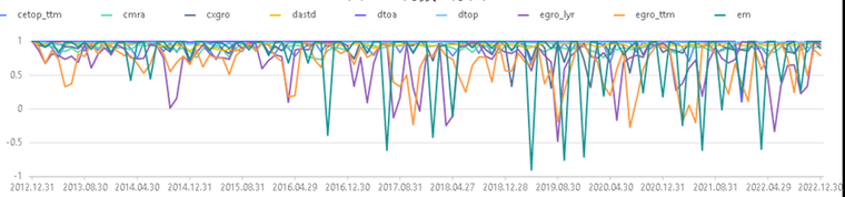
Figure 10. Figure 2-8 Monthly Time Series of the FSC Factors whose FSC remains above 0.8 most of the time are generally considered to have high stability. In the figure above, all factors except em, dastd, and dtoa exhibit good stability.
-
Step 3: Plot the monthly IC time series to evaluate factor consistency. An IC value above 0.03 is considered to indicate that the factor has consistent or inverse fluctuation patterns with the market, and thus the factor has some effectiveness.
tmp1 = select record_date,valueType.regexReplace("_stat","") as valueType,
              abs(ic) as ic from factorsValid
tmppivot1 = select ic from tmp1 pivot by record_date,valueType
tbic = sql(select = sqlCol(tmppivot1.columnNames()[2:10]),from = tmppivot1).eval()
baseline = take(0.03,(shape tbic)[0])
plot(table(tbic,baseline),tmppivot1.record_date,
    extras={multiYAxes: false},title = "Monthly Time Series of Factor IC")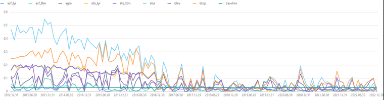
Figure 11. Figure 2-9 Monthly Time Series of Factor IC It can be observed that the atvr (Annualized Traded Value Ratio) factor maintained a strong correlation before 2017, while from 2018 to 2022 the eight factors exhibited periodic fluctuations.
-
Step 4: Plot the factor t-statistics to evaluate factor effectiveness.
tmp2 = select record_date,valueType.regexReplace("_stat","") as valueType,
              tstat from factorsValid
tmppivot2 = select tstat from tmp2 pivot by record_date,valueType
tbstat = sql(select = sqlCol(tmppivot2.columnNames()[11:20]),from = tmppivot2).eval()

baseline_neg = take(-0.03,(shape tbstat)[0])
baseline_pos = take(0.03,(shape tbstat)[0])
plot(table(tbstat,baseline_neg,baseline_pos),tmppivot2.record_date,
    extras={multiYAxes: false},title = "Monthly Time Series of Factor t-statistics")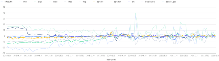
Figure 12. Figure 2-9 Monthly Time Series of Factor t-statistics In the figure, the t-values of most factors are far from the baselines of 0.03 and -0.03. For example, dastd and cmra: one is significantly above 0.03, and the other is significantly below -0.03. It can therefore be concluded that before 2018, these two factors exhibited significant positive and negative correlations with the market, respectively.
2.5 Multi-Factor Synthesis
Based on the Level-3 factors and their effectiveness identification results, the factors can then be combined. The synthesis methods are based on widely-adopted industry research models, such as the equal-weight method and the historical information method.
-
Equal-weight method: The corresponding Level-3 factors are equally weighted to synthesize Level-2 and Level-1 factors. For example, assign a weight of 1/2 to each of the ABS and ACF_TTM factors to synthesize the Earnings Quality factor.
-
Historical return weighting method (ir): The Level-3 factor returns from the single-factor model test are standardized to obtain the weighting coefficients, which are then used to synthesize Level-2 factors.
-
Information coefficient ratio method (ic_ir): Factors are synthesized using the IC values obtained from factor testing. For example, let X be the K × T IC matrix of K factors over the past T cross-sectional periods, let x̄ be the row mean of matrix X, and let V be the K × K covariance matrix of X. Then V-1x̄ can be taken as the weight to synthesize factors at each level.
The corresponding function for factor synthesis in this article is getFSLevelFactor. In this function, the Level-2 factor names in firstFactors must correspond one-to-one with the Level-2 factor names in secondFactors; the Level-3 factors in secondFactors must correspond to the field names of the input factor table factorsTable (with case-sensitive matching).
Input:
         factorsTable     NULL  (Default)    (Full factor table returned by the getRegTable function)
         factorsValid     NULL  (Default)    (Single-factor return and test table returned by the getFactorsValidation function)

         firstFactors     NULL               JSON defining the relationships between Level-1 and Level-2 factors
         secondFactors    NULL               JSON defining the relationships between Level-2 and Level-3 factors
         normlizing       true               Whether to standardize the synthesized factors
         method           "equal"            Equal weighting; "ir" Historical return weighting; "ic_ir" Method for synthesizing factors
         level            "S", "F"           Specifies the level of factors to synthesize:
                                             "S" for Level-2 style factors and "F" for Level-1 style factors

Output:
         factorsTable                        Returns a table of synthesized style and industry factors
                                             based on the specified relationships, which can be directly used in regression models
st = 2022.01.03
et = 2023.01.02
normlizing = true
scaling = true
decap = true
industry_method = 'CITIC'
industry_weighted = true
Factors = getAllFactors(st= st,et = et, normlizing = normlizing,scaling = scaling,
decap = decap,industry_method = industry_method,
industry_weighted = industry_weighted)
select * from Factors limit 100
// Handle missing values in the raw factor wide table.
fTable = getRegTable(factorsTable = true,tbName = Factors,st= st,et = et,
normlizing = normlizing ,scaling = scaling ,
decap = decap,industry_method = industry_method,
industry_weighted = industry_weighted)
// Factor validity test
// Obtain validity, consistency, and stability checks for single-style factors.
factorsValid = getFactorsValidation(factorsTable = true,tbName = Factors,st = st,
et = et , normlizing = normlizing,scaling = scaling,
decap = decap,industry_method = industry_method,
industry_weighted = industry_weighted)
factorsValid
update factorsValid set tstat = abs(tstat)
// Compute FSC
tmp = select record_date,valueType.regexReplace("_stat","") as valueType,
fsc from factorsValid
tmppivot = select fsc from tmp pivot by record_date,valueType
tbfsc = sql(select = sqlCol(tmppivot.columnNames()[11:20]),from = tmppivot).eval()
plot(tbfsc,tmppivot.record_date,extras={multiYAxes: false},title = "Monthly Time Series of Factor FSC")
// Compute IC
tmp1 = select record_date,valueType.regexReplace("_stat","") as valueType,
abs(ic) as ic from factorsValid
tmppivot1 = select ic from tmp1 pivot by record_date,valueType
tbic = sql(select = sqlCol(tmppivot1.columnNames()[2:10]),from = tmppivot1).eval()
baseline = take(0.03,(shape tbic)[0])
plot(table(tbic,baseline),tmppivot1.record_date,
extras={multiYAxes: false},title = "Monthly Time Series of Factor IC")
// Compute t_stat
tmp2 = select record_date,valueType.regexReplace("_stat","") as valueType,
tstat from factorsValid
tmppivot2 = select tstat from tmp2 pivot by record_date,valueType
tbstat = sql(select = sqlCol(tmppivot2.columnNames()[11:20]),from = tmppivot2).eval()
baseline_neg = take(-0.03,(shape tbstat)[0])
baseline_pos = take(0.03,(shape tbstat)[0])
plot(table(tbstat,baseline_neg,baseline_pos),
tmppivot2.record_date,extras={multiYAxes: false},
title = "Monthly Time Series of Factor t_stat")As shown in the results of the synthesized Level-1 factors below, factors such as 'abs', 'acf_ttm', 'acf_lyr', 'vsal_ttm', and 'vsal_lyr' are synthesized into Level-1 factors such as Quality.
Before factor synthesis:

Synthesized Level-1 factors:

2.6 Multi-Factor Synthesis with User-Defined Factors
2.6.1 User-Defined Factor Preprocessing
-
Preprocess the existing factor data by calling functions such as
winsorizedandstandardizedto winsorize and standardize the style factors. -
Handle missing values in the preprocessed factor data to prevent missing factor values from affecting the results of the regression model.
Assuming the final factor table is Factors, you can call the getRegTable function to handle missing values.
fTable= getRegTable(factorsTable = true,tbName = Factors,st= st,et = et)2.6.2 Single-Factor Model Testing for User-Defined Factors
Assuming the final factor table is Factors, you can call the getFactorsValidation function to perform single-factor model testing and further screen for effective factors.
factorsValid= getFactorsValidation(factorsTable = true,tbName = Factors,st= st,et = et)2.6.3 Multi-Factor Synthesis Using User-Defined Factors
After mapping the user-defined factors to their corresponding Level-1 and Level-2 factors, use the getFSLevelFactor function to synthesize the Level-1 and Level-2 factors from the user-defined factors.
getFSLevelFactor(fTable,factorsValid,firstFactors,secondFactors,false , "ir",level = "F")
getFSLevelFactor(fTable,factorsValid,firstFactors,secondFactors,false , "ir",level = "S")
3. Return and Risk Model Based on DolphinDB
After synthesizing Level-1 factors, a return and risk model can be built based on the complete set of factors, including all factor returns, bias statistics, and goodness of fit. Bias statistics measure the difference between the risk predicted by the model and the actual risk. Goodness of fit reflects how well the full set of factors explains market returns. A goodness-of-fit value closer to 1 indicates greater model robustness and accuracy.
The corresponding function for the return and risk model in this article is
getRetTable. It calculates and returns the factor risk
covariance matrix, the idiosyncratic return covariance matrix, bias_statistic,
stR2, t-statistics, and factor returns. These return values can be
used to assess factor risk and idiosyncratic risk, as well as the accuracy of the
model’s risk estimates (bias) and the model’s explanatory power
(stR2).
/* getRetTable
Input:
         facTable    NULL (Default)    Full factor table (returned by the getFSLevelFactor function)
         adjust      true (Default)    Whether to apply Newey-West adjustment
         shrink      true (Default)    Whether to apply Bayesian shrinkage
         eigenfactor true (Default)    Whether to apply eigenfactor adjustment
Output:
         factorsRetTable
*/
3.1 Build a Multi-Factor Model with WLS
First, use the function getAllFactorValidate to build a moving WLS multi-factor regression model.
/* getAllFactorValidate
Aggregate function for obtaining moving WLS multi-factor regression statistics
Input:   y    dependent variable
         x    independent variable
         w    weight
Output:
         wls stat "beta","tstat","R2","AdjustedR2","Residual"
*/
After building the multi-factor regression model, use the getRetTable function to calculate the following model evaluation metrics:
-
stR2: This value is the Studentized R2 defined in the multi-factor model, and it is calculated as follows: , where rn is the excess return of stock n, εn is the residual of the cross-sectional regression, wn is the weighting of the stock, Hnn is the n-th diagonal element of H = X(X'X)-1X', and X is the factor exposure matrix.
-
t-test: This value is the standard t-statistics, used to measure the statistical significance of the regression coefficients.
Bias statistic (bias_statistic): This statistic is a general measure of the model’s prediction accuracy. Intuitively, it is the ratio of actual risk to predicted risk. Let Rnt be the return of portfolio n at time t, and σnt be the volatility forecast at time t, the formula is . It can be understood as standardizing the volatility of Rnt. If the prediction is accurate, the standard deviation of bnt is 1. The bias statistic of portfolio at time is given by:
.where T is the total number of cross-sectional time periods. Under the assumption that returns are normally distributed, the 95% confidence interval for the bias statistic Bn is:
.
Therefore, when the observed Bn is close to 1, we can preliminarily conclude that the model's predicted values are relatively accurate.
-
Q Statistic (Q_statistic): Calculated based on the bias statistic, this metric penalizes both underfitting and overfitting. The Q statistic is calculated as follows: .
3.2 Risk Adjustment
After constructing the multi-factor regression model, solving for the stock return covariance matrix in the multi-factor model requires solving for the factor return covariance matrix Vf and the idiosyncratic return covariance matrix Δ. However, the estimates of Vf and Δ obtained from the sample are biased. Therefore, covariance adjustments need to be applied to the factor return risk matrix and the idiosyncratic return covariance matrix separately.
3.2.1 Factor Return Risk Adjustment
3.2.1.1 Newey-West Adjustment
There are two main reasons why a multi-factor model must apply Newey-West covariance adjustment:
-
The multi-factor model is daily-frequency, while the risk prediction model is monthly-frequency. Therefore, the daily covariance matrix must be converted into a monthly covariance matrix by a scale transformation, and this process must account for the autocorrelation of daily factor returns.
-
In practice, factor returns predicted by a multi-factor model often exhibit serial correlation. In this case, the sample risk matrix is not a consistent estimator of the true return risk matrix (a consistent estimator converges to the true value as the sample size increases, which helps in calculating the estimation error of the estimator). Therefore, the factor return risk matrix Vf, which is distorted by the q-th order serial correlation in the computed daily returns, needs to be adjusted.
The Newye_West function implements the Newey-West covariance adjustment described in this section. It is called by getRetTable when adjust=true.
/* Newye_West
Newye_West adjustment yields the covariance matrix
Input:
         ret                    return table
         q                      autocorrelation order of returns
Output:
         cov                    covariance matrix adjusted by Newye_West
*/
The main implementation steps of the above interface are as follows:
-
Assume that follows an process. A simple validation can first be performed based on the moving average process, as shown below.
.
Here, denotes the sample covariance matrix without considering autocorrelation, while denotes the autocovariance matrix obtained from the return vector at the current period and the return vector lagged by i periods. However, is not symmetric, so and must appear as a pair for each lag .
Apply the Bartlett weighting coefficient to the adjustment of . The coefficient is inversely related to the lag: the longer the lag between return vectors, the lower the weight assigned to . It can be shown that the sample risk matrix Vf obtained after this correction is a consistent estimator of the true risk matrix and is positive semidefinite.
.
3.2.1.2 Eigenfactor Adjustment
Let denote the factor covariance matrix K×K of Vf. Using eigendecomposition, Vf can be expressed in diagonal form as , where U0 is the eigenvector rotation matrix composed of the eigenvectors corresponding to the eigenvalues of Vf.
In business terms, suppose there are N stocks. Each column of U0 is an N*1 eigenfactor portfolio weight vector. Using these weights, an eigenfactor portfolio is constructed (the eigenfactor portfolio is derived from eigenvectors), where each diagonal element of D0 is the volatility risk of the corresponding eigenfactor portfolio. The eigenfactor portfolio is of great significance in optimal portfolio construction:
-
The eigenfactors are independent of each other, and the covariance between any two eigenfactors is zero.
-
The eigenfactor with the smallest variance represents the portfolio constructed with the objective of minimizing portfolio variance, while the eigenfactor with the largest variance represents the portfolio constructed with the objective of maximizing portfolio variance.
However, direct eigendecomposition introduces bias; the lower the risk of an eigenfactor portfolio, the larger the bias. Therefore, eigenfactor adjustment is necessary. The eigenCovAdjusted function implements the eigenfactor adjustment described in this section. It is called by getRetTable when eigenfactor=true.
/* eigenCovAdjusted
eigenCovAdjusted adjusts the style factor covariance matrix
Input:
         cov                    factor return covariance matrix
         M                      Monte Carlo simulation: number of resamples

Output:
         cov                    covariance matrix adjusted by eigenCovAdjusted
*/
The main implementation steps of the above interface are as follows:
-
First, use Monte Carlo simulation to construct a biased covariance matrix relative to the “true” covariance matrix, referred to as the simulated covariance matrix .
-
Generate K×T multivariate normal factor returns bm with mean 0 and covariance D0, where each row represents the return series of an eigenfactor. Thus, represents the simulated factor return time series, and its corresponding covariance matrix is the simulated covariance matrix .
-
Further eigendecomposition yields the simulated eigenfactor covariance matrix .
-
-
The simulated eigenfactors Um above are obtained using the sample covariance matrix Vf as the true factor return covariance matrix. Here, Vf can be regarded as the true value of Vm, while Vm is an unbiased estimator of Vf. Therefore, the simulated “true covariance matrix” is .
-
Calculate the scaling factor / bias adjustment coefficient. Based on the diagonal elements and of and , respectively, the bias adjustment coefficient can be calculated , where M is the total number of bootstrap simulations.
-
Adjust the eigenfactor matrix obtained from the sample data as follows: . Here, v is a diagonal matrix generated from v(k), yielding the final adjusted covariance matrix .
3.2.2 Stock-Specific Idiosyncratic Return Risk Adjustment Based on Bayesian Shrinkage
Bayesian shrinkage is a common technique for combining prior information with sample estimates. The main reason for applying Bayesian shrinkage adjustment is that idiosyncratic volatility computed from in-sample data using a multi-factor risk model has poor out-of-sample persistence. Extremely high or low individual stock volatility may exhibit mean reversion, causing volatility to be overestimated or underestimated.
The BayesShrinkage function implements the Bayesian shrinkage described in this section. It is called by getRetTable when shrink=true.
/* BayesShrinkage
BayesShrinkage adjusts idiosyncratic volatility
Input:
         cov                    idiosyncratic return covariance matrix
         weight                 market capitalization weight
         q                      λ_F shrinkage coefficient

Output:
         cov                    covariance matrix adjusted by BayesShrinkage
*/
The implementation steps of the above interface are as follows:
-
Calculate the sample estimate—the idiosyncratic return risk obtained from WLS predictions.
Calculate the prior-first select all stocks in the same market-capitalization group as the target stock, and then calculate the market-capitalization-weighted average of the idiosyncratic return volatility.
Here, the multi-factor risk model divides all stocks into ten market-capitalization buckets. sn denotes the corresponding market-capitalization bucket, is the idiosyncratic return volatility of the n stocks in the same market-capitalization bucket sn, and wn denotes the market-capitalization weight of the n stocks.
Apply Bayesian shrinkage (shrinking the sample estimate toward the prior) to compute the posterior estimate.
vn is the weight assigned to the prior during shrinkage (called the shrinkage intensity coefficient). The specific formula is as follows:
where N(sn) is the total number of stocks in the current market capitalization bucket, is the degree of deviation between the sample idiosyncratic volatility and the prior, is the standard deviation of that deviation within the bucket sn, and q is the empirical shrinkage coefficient, which controls whether more weight is placed on the within-bucket standard deviation or on the deviation of a stock from the bucket mean. As increases, indicating a greater deviation in the volatility of the target stock’s idiosyncratic returns, the sample estimate becomes less reliable. Therefore, a higher prior weight vn is assigned.
3.3 Return Risk Model Demonstration Based on DolphinDB
The following illustrates the return-risk model obtained using
getRetTable, along with the corresponding model evaluation
metrics, including R2, t-statistics, Bias statistic, etc. The
following plot shows the model's Studentized R2. From 2012 to
2022, the model's explanatory power ranges from a minimum of 5% to a maximum of
84%, with an average of 37%, indicating relatively strong explanatory power.
// Level-1 factor return regression
retOut1 = getRetTable(facTable1,adjust = true)
// adjust uses Newey-West covariance adjustment. Use this method when market returns exhibit serial autocorrelation.
retOut1 = getRetTable(facTable1,adjust = false,shrink = false)
// shrink uses Bayesian shrinkage to adjust idiosyncratic risk. Recommended.
retOut1 = getRetTable(facTable1,adjust = true,shrink = true)
 // Idiosyncratic risk is adjusted using Bayesian shrinkage.
retOut1 = getRetTable(facTable1,adjust = true,shrink = true,eigenfactor = true)
// Factor risk is adjusted using eigenfactor adjustment. Use this method when market correlations are high.
retOut1 = getRetTable(facTable1,adjust = true,shrink = true,eigenfactor = true)
// In summary, it is recommended.
retOut1 = getRetTable(facTable1,adjust = false,shrink = true,eigenfactor = true)
// In summary, it is recommended.
retOut1 = getRetTable(facTable1,adjust = false,shrink = true,eigenfactor = true)
// In summary, it is recommended.
retOut1 = getRetTable(fTable,adjust = false,shrink = true,eigenfactor = false)
// In summary, it is recommended.
undef(`retOut)
retOut = getRetTable(facTable1,adjust = true,shrink = false ,eigenfactor = false)
// In summary, it is recommended.
retOut1.stock_risk[string(2022.12.30)]   // Covariance matrix of idiosyncratic returns as of 12.30
retOut1.fac_risk[string(2022.12.30)]     // Risk factor covariance matrix as of 12.30
retOut1.R2                               // R2
retOut1.res                              // Idiosyncratic returns
retOut1.tstat                            // t-statistics
retOut1.fac_ret                          // Factor returns
retOut1.bias                             // Bias statistic

plot(retOut1.R2.stR2,retOut1.R2.record_date,"Monthly Time Series of Studentized R²")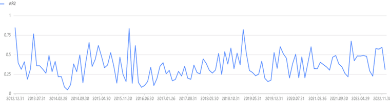
4. Multi-Factor Model Applications Based on DolphinDB
4.1 Predict Individual Stock Returns
There are various approaches to forecasting individual stock returns. Economic or other models can be used to forecast factor returns for period t+1 based on the time series of fm,t, fi,t, fs,t, and un,t, which can then be used to derive the predicted individual stock returns. Since multi-factor models are constructed without considering investability constraints, predicted returns based on multi-factor models have limited practical applications. To simplify the modeling process, DolphinDB provides a one-period-ahead prediction model based on the multi-factor risk model.
Note: By the end of period t, the period-t stock return rn,t, as well as xn,i,,t-1, xn,s,t-1, xn,i,t, and xn,s,t, are already available. Substituting rn,t, xn,i,t-1, and xn,s,t-1 into the model yields fm,t, fi,t, fs,t, and un,t, which have one-period-ahead predictive power. Combining these with the values xn,i,t and xn,s,t at the end of period t yields the predicted stock returns for period t. Compared with direct multi-factor modeling and prediction, this modeling approach gives the estimated fm,t, fi,t, fs,t, and un,t partial one-period-ahead predictive power.
Accordingly, the getPredicOut function is provided to forecast
individual stock returns based on the above model. Assuming that the prediction
period is the last period of the full factor table (the data for the first
t-1 periods in the full factor table must be complete), the expected
factor returns can be calculated from the factor exposures at the beginning of
the current month (i.e., the end of the previous month) to predict the stock
returns at the end of the current month. The function returns the factor
covariance matrix (factor risk), the idiosyncratic return covariance matrix
(idiosyncratic risk), the goodness of fit R2, the adjusted
goodness of fit adR2, the Studentized R2
stR2, and the tstat statistic of the prediction
model to evaluate the model's prediction accuracy.
/* getPredicOut
Input:
         facTable             NULL (Default)               (Required) Factor table
Output:
         predictRetTable
*/
The following script calls the getPredicOut function:
predictOut = getPredicOut(facTable1)
pr = select * from predictOut.predict_ret    // Predict the return of the last period using current-period factor exposures.
predictOut.R2                               // Prediction model R2
predictOut.res                              // Prediction model idiosyncratic returns
predictOut.tstat                            // Prediction model t-statistics
predictOut.fac_ret                          // Prediction model factor returns
predictOut.bias                             // Prediction model bias statistic
Note: The output of predictOut = getPredicOut(facTable1) is extensive. To inspect the results, it is recommended to persist them first, or retrieve only a smaller subset. In addition to predicted returns, the results include R2, t-statistics, monthly factor returns, idiosyncratic returns, risk factor covariance matrix, idiosyncratic risk table, and bias statistic.
4.2 Portfolio Weight Optimization
Portfolio weight optimization plays a crucial role in multi-factor models. Portfolio weight optimization quantifies a portfolio's risk profile, helping investment managers see where its returns and risk exposures come from. The weight-optimization objective function can take various forms. For example, it can minimize portfolio risk subject to a minimum predicted return, minimize portfolio risk subject to a minimum current-period return, maximize predicted return subject to a maximum risk, maximize current-period return subject to a maximum risk, and so on. The process of portfolio weight optimization consists of two elements: the objective function and the constraints.
4.2.1 Objective Function
Assume that the idiosyncratic return of each stock in the portfolio is uncorrelated with the common factor returns, and that the idiosyncratic returns of individual stocks are also uncorrelated with each other. Therefore, if w represents the weights of the stocks in the portfolio, the risk matrix of portfolio P can be
expressed as: .
4.2.2 Constraints
-
Industry Neutrality
Industry neutrality means that the industry allocation of the long portfolio is consistent with that of the hedging benchmark. The purpose of industry-neutral allocation is to eliminate the influence of industry factors on strategy returns and to focus only on the excess returns of individual stocks within industries. Let H be the industry factor dummy matrix of the sample stocks, and h be the corresponding weights of the 30 industries in the CSI 300. Then the industry-neutral weight w satisfies: .
-
Style Factor Neutrality
Style factor neutrality means that the style factor risk exposure of the long portfolio relative to the hedging benchmark is zero. The purpose of style-factor-neutral allocation is to eliminate the portfolio's risk exposure to market style factors, so that the portfolio's returns come mainly from alpha returns rather than from a specific market style. Let X be the cross-section of factor loadings for the k-th factor in the sample, and wbench be the corresponding CSI 300 index weight. Then the style-neutral weight w for factor k satisfies: .
-
Cash Neutrality
Cash neutrality means that the long and short market values are equal, leaving no directional exposure. Then the cash-neutral weight w satisfies: .
-
Minimum Predicted Return
Imposing a minimum predicted return is one of the constraints in multi-factor portfolio weight optimization. Its purpose is to ensure a minimum return level, help control risk, avoid irrational allocations, and maintain model consistencyThis makes the portfolio more consistent with investment objectives and risk preferences, and improves the overall stability and predictability of the portfolio. Suppose rmin is the benchmark return. Then the portfolio weight w should satisfy: .
4.2.3 Implement Portfolio Weight Optimization
This section presents an optimization method that minimizes predicted returns and portfolio risk subject to industry and style neutrality constraints. The corresponding function getOptimizeWeights implements the following optimization objective. The deIndustry and deStyle parameters can be used to specify whether to impose industry and style neutrality constraints, respectively.
/* getOptimizeWeights
Aggregate function in portfolio weight optimization
Input:
         covf              Factor return covariance matrix
         delta             Idiosyncratic return covariance matrix
         st                2022.01.03(Default)
         et                2023.01.02(Default)
         ret               Expected return
         r                 0.05                              Set minimum predicted return
         tbName            Factor exposures
         deIndustry        true                             Industry neutrality
         deStyle           true                             Style neutrality

Output:
         weightTable       Returns the predicted asset allocation weights
*/
Using the getOptimizeWeights function, the following script implements risk minimization subject to a minimum return:
optionCode = exec stock_code from getPredicOut(facTable1).predict_ret
             order by return_day desc limit 20
// Preliminary screening of stock1
optionCode = exec stock_code from getPredicOut(facTable2).predict_ret
             order by return_day desc limit 20

// Model with return constraint and risk minimization
portWeight1 = getOptimizeWeights(facTable = facTable1,retOut = retOut1,
                                 st = st,et = et, method ="minRiskControlRet",
                                 r = 0.05,optionCode = optionCode)
// Get portfolio weights
portWeight2 = getOptimizeWeights(facTable = facTable2,retOut = retOut2,
                                 st = st,et = et, method ="minRiskControlRet",
                                 r = 0.05, optionCode = optionCode)

index_code = '000300'
CodePre = set(exec stock_code from getPredicOut(facTable1).predict_ret
              order by return_day desc limit 200)
 // Preliminary screening of stock2
CodeWeight = set(exec stock_code
                from getBenchMark(st=st,et=et,code = index_code)
                where i_weight != 0)
CodeFac =set(exec stock_code from facTable1 )
optionCode = (CodePre&CodeWeight&CodeFac).keys()
portWeight3 = getOptimizeWeights(facTable = facTable1,retOut = retOut1,
                                 st = st,et = et, method ="minRiskControlRet",
                                 r = 0.005,deStyle = true,optionCode = optionCode)
// Obtain the weight combination and achieve zero exposure to style risk.
portWeight3 = getOptimizeWeights(facTable = facTable1,retOut = retOut1,st = st,
                                 et = et, method ="minRiskControlRet",r = 0.005,
                                 deIndustry = true,optionCode = optionCode)
// Obtain the weight combination and achieve zero exposure to industry risk.
portWeight4 = getOptimizeWeights(facTable = facTable2,retOut = retOut2,st = st,
                                 et = et, method ="minRiskControlRet",r = 0.05,
                                 optionCode = optionCode)
4.3 Asset Allocation Evaluation
4.3.1 Evaluate Ex-Post Asset Allocation
Ex-post asset allocation refers to the allocation of assets based on actual historical return data after those returns become available. This process occurs after investment decisions are made and reallocates assets based on the observed historical return data. Therefore, by evaluating the bias of an existing index using the market-capitalization or equal-weight method, the bias statistic and Q statistic of a specified portfolio can be calculated to evaluate the ex-post asset allocation.
-
Factor (portfolio) Bias
-
Asset (portfolio) Bias
Use the getFacSpecialBias function to calculate the bias statistics of the ex-post asset allocation to evaluate it.
/*
Get the time-series Bias statistics of factors and the idiosyncratic return statistics of individual stocks
Input:
         retOut   The result returned by the getRetTable() function
         index_name   Index code
         method   Equal-weight or float market-capitalization method: 'equal', 'float_market'
Output:
         Bias statistics
*/
4.3.1.1 Ex-Post Factor Portfolio Evaluation
In the following script, assuming facTable1 is the table of all factor portfolios actually invested, we use getFacSpecialBias to calculate the bias of factor returns and the bias of idiosyncratic returns to evaluate the ex-post factor portfolios.
// Factor portfolio
retOut = getRetTable(facTable1,adjust = true,shrink = false ,eigenfactor = false)

// Get the time-series Bias statistic values of all factors and all individual stocks.
biasOut = getFacSpecialBias(retOut)

// Factor Bias
tmpfBias = select bias_stat from biasOut.fac_bias pivot by record_date,valueType
tmpfBias = tmpfBias[23:]
tbfBias = sql(select = sqlCol(tmpfBias.columnNames()[1:9]),from = tmpfBias).eval()

plot(tbfBias,tmpfBias.record_date,extras={multiYAxes: false},
     title = "Time Series of Factor Model Factor Bias Statistics")
plot(tbfBias,tmpfBias.record_date,extras={multiYAxes: false})

code0 = parseExpr("rowAvg("+ concat(tmpfBias.columnNames()[1:],',') + ")")
avgfBias =  sql(select = sqlColAlias(code0,'avg_bias_stat'),from = tmpfBias ).eval()
plot(avgfBias,tmpfBias.record_date,extras={multiYAxes: false},
     title = "Time Series of Factor Mean Bias Statistics")
plot(avgfBias,tmpfBias.record_date,extras={multiYAxes: false})

// Idiosyncratic  Bias
tmpsBias = select mean(bias_stat) from biasOut.stock_bias group by record_date
tmpsBias = tmpsBias[23:]

plot(tmpsBias.avg_bias_stat,tmpsBias.record_date,
     extras={multiYAxes: false},title = "Time Series of Factor Model-Specific Risk Bias Statistics")
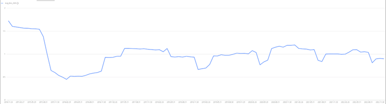
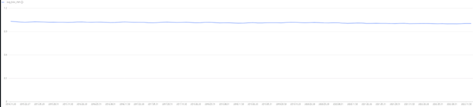
In the following figures, we plot the time-series bias statistics of the factors and the mean factor bias statistics for the ex-post multi-factor model. For the CNLT monthly model, the bias statistics of the eight style factors all remain near 1 over the long term, with a mean of 0.9962, indicating that the model's factor risk estimates are relatively accurate. The mean factor bias statistics also remain stable near 1 over the long term. Therefore, from both the factor risk perspective and the idiosyncratic risk perspective, the model's estimates are relatively accurate.
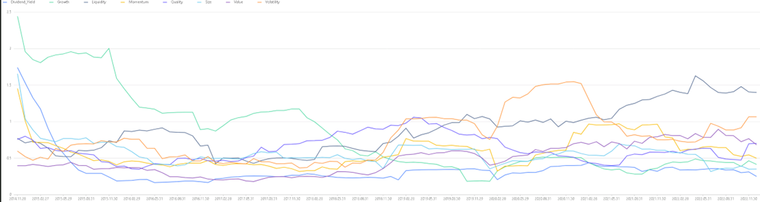
Mean factor bias curve:
Factor model idiosyncratic risk bias statistic evaluation:
4.3.1.2 Ex-Post Portfolio Evaluation
Taking the equal-weighted portfolio of the CSI 300 Index as an example, we use getFacSpecialBias to calculate its Bias statistics and plot the Bias of the CSI 300 equal-weighted portfolio as shown below.
/*Simple asset allocation evaluation*/
// Calculate the Bias statistics of the index allocation.
tmpIndexbiasbn = getFacSpecialBias(retOut,'000300','equal').stock_bias
tmpIndexBias = select wavg(bias_stat,weight) from tmpIndexbiasbn group by record_date
plot(tmpIndexBias.wavg_bias_stat,tmpIndexBias.record_date,extras={multiYAxes: false})
tmpIndexbiasbn = getFacSpecialBias(retOut,'000300','float_market').stock_bias
tmpIndexBias = select wavg(bias_stat,weight) from tmpIndexbiasbn group by record_date

plot(tmpIndexBias.wavg_bias_stat,tmpIndexBias.record_date,extras={multiYAxes: false})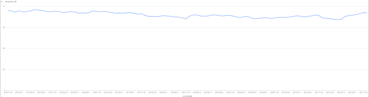
In the figure above, the mean bias is 1.08, indicating that the risk prediction for the CSI 300 equal-weighted asset allocation is fairly consistent with the actual risk.
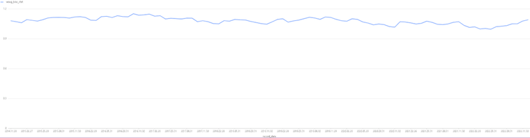
In the figure above, the mean bias is 1.08, indicating that the risk prediction for the CSI 300 float market-capitalization-weighted asset allocation is also fairly consistent with the actual risk.
4.3.2 Evaluate Ex-Ante Model Asset Allocation
Ex-ante asset allocation refers to asset allocation based on model predictions and assumptions before actual return data becomes available. This process occurs before investment decisions are made and allocates assets based on model predictions, investor objectives, constraints, and other factors. Using portfolio weights derived from an optimization objective or given in advance, we can calculate the bias statistic and Q statistic of a specified portfolio to examine the rationality of the specified asset allocation weights or evaluate the quality of the optimized weights.
Use the getPortfolioAccuracy function to evaluate ex-ante asset allocation portfolios.
/* getPortfolioAccuracy
Calculate the time-series Bias statistic and Q-statistic of a portfolio
Input:
         facTable          NULL   (Default)   Full factor regression table (returned by the getFSLevelFactor function)
         retOut            NULL  (Default)   Full factor return table (returned by the getRetTable function)
         st                2022.01.03(Default)
         et                2023.01.02(Default)
         index_code        Specified portfolio       '000300', '399101'
         method            Weighting method       "float_value" for float market-capitalization weighting, "equal" for equal weighting
Output:
         accuracyTable
         */
Taking the equal-weighted portfolio of the CSI 300 Index as an example, the getPortfolioAccuracy function can be used to calculate the deviation of the ex-ante predicted portfolio. The mean Bn statistic is 0.335, which is less than 1. However, the bias result here is related to the portfolio weights obtained from the ex-ante prediction. This indicates that the equal-weighted portfolio of the CSI 300 Index has weak predictability of future risk, suggesting that the asset allocation should be reconsidered.
/* Calculate the Bias and Q statistics of the prediction model. */
index_code = '000300'
st = 2022.01.03
et = 2023.01.02
outAccuracy = getPortfolioAccuracy(st,et,facTable1,retOut,index_code,'equal')
outAccuracy = outAccuracy[2:]
baseline = take(1,(shape outAccuracy)[0])
plot(table(outAccuracy.bias_statistic,baseline),outAccuracy.record_date, extras={multiYAxes: false})
mean(outAccuracy)
5. Implementation and Application of a Multi-Factor Risk Model Based on DolphinDB
This chapter describes in detail how to use the multi-factor risk model module, covering environment configuration, data preparation, and methods for invoking calculations.
5.1 Environment Preparation
From the RiskFactors folder in the attachment, place the helper folder, RiskFactorsCal.dom, and RiskFactorsModel.dom in the [home]/modules directory. The [home] directory is determined by the system configuration parameter home and can be obtained using the getHomeDir function.
For more details on module usage, see Modules.
5.2 Data Preparation
This document provides a factor mapping table for factor testing (factor_table.xlsx). The data contains all database table structures and required fields involved in building the RiskFactors multi-factor model. For your data, ensure that the table field names in the current data match the module field names. For convenience, this tutorial provides an auxiliary module, RiskFactorsPrepare.dos, to help unify field names. Before calling the auxiliary module, place it in the same directory as RiskFactors.
The auxiliary module contains the following types of functions:
-
The
prepareMockDatafunction generates simulated test data. startTime and endTime specify the start and end times of the desired data. -
The
prepareModelDatafunction generates factor validity test results and factor synthesis results based on local data. -
The
plotFactorsValidationfunction plots the corresponding results based on the factor validity test results. -
The
Assessmentfunction is an asset allocation evaluation function.
The methods for loading the module and data are as follows:
use RiskFactors::RiskFactorsCal
use RiskFactors::RiskFactorsModel
use RiskFactors::helper::RiskFactorsPrepare

startTime,endTime = 2018.01.01, 2023.01.01
prepareMockData(startTime,endTime)
5.3 RiskFactors Module Usage Examples
For user convenience, RiskFactorsTest.dos in the attachment provides an example of the complete workflow for building the RiskFactors multi-factor model. The scripts provided below can all reference RiskFactorsTest.dos.
5.3.1 Factor Calculation
To calculate a style factor, call the function formed by `get` plus the style factor name. Taking the ABS factor as an example, it can be calculated by calling the getAbs() function as follows:
// Get raw style factors,some sample codes:
getAbs(startTime = 2022.01.03,endTime = 2023.01.02)
After calculating a single style factor, call functions such as getIndustry and getIndustryFactor to obtain industry factors. Taking the CITIC Level-1 industry classification as an example, the calculation method is as follows:
// Get raw industry factors,some sample codes:
getIndustry(startTime = 2022.01.01,endTime = 2023.01.02,method = 'CITIC')
// Get Industry Factor Weights,some sample codes:
getIndustryWeighted(startTime = 2022.01.03,endTime = 2023.01.02,method = 'CITIC')
// Get weighted industry factors
getIndustryFactor(startTime = 2022.01.03,endTime = 2023.01.02,method = 'CITIC')
5.3.2 Factor Synthesis
The factor synthesis process in the RiskFactors module is relatively complex and must be handled step by step along the following pipeline:
-
Use
getAllFactorsto obtain all factors. -
Use
getRegTableto handle missing values in the raw factor table. -
Use
getFactorsValidationto validate all factor tables. -
Use
getFSLevelFactorto synthesize factors.
To facilitate further construction of the RiskFactors model, the workflow described above can be executed in a unified manner using the prepareModelData function. For example, to generate a Level-1 factor table for the period from January 3, 2022 to January 2, 2023, with the raw factors market-capitalization-weight standardized and winsorized, the CITIC Level-1 industry classification applied, and Level-1 factors synthesized using equal weighting, use the following script. If factor synthesis is not required, set merge_level=NULL:
st = 2022.01.03
et = 2023.01.02
normlizing = true
scaling = true
decap = true
// also you can choose industry_method = 'SW_2021'
industry_method = 'CITIC'
industry_weighted = true
// Get ALL FIRST level of factors and factor Validation table
factorsValid,facTable1=prepareModelData(st,et,normlizing,scaling,decap,
                                        industry_method,industry_weighted,
                                        merge_method="equal",merge_level="F")

select * from facTable1 limit 100
In addition, using the factor validity metrics in factorsValid obtained above, you can further evaluate factor effectiveness. The usage is as follows:
x,y=plotFactorsValidation(factorsValid,"fsc")
plot(x,y,extras={multiYAxes: false},title = "Monthly Time Series of Factor FSC")

x,y=plotFactorsValidation(factorsValid,"ic")
plot(x,y,extras={multiYAxes: false},title = "Monthly Time Series of Factor IC")

x,y=plotFactorsValidation(factorsValid,"t")
plot(x,y,extras={multiYAxes: false},title = "Monthly Time Series of Factor t-statistics")
5.3.3 Factor Model
Use the getRetTable function to build a RiskFactors multi-factor model from factor tables. The following example assumes that market returns exhibit serial autocorrelation, market factors are closely correlated, and adjustment for idiosyncratic risk is required:
retOut1 = getRetTable(facTable1,adjust = true,shrink = true,eigenfactor = true)

// the output of getRetTable function
// the idiosyncratic return covariance matrix for 12.30
retOut1.stock_risk[string(2022.12.30)]
// risk factor covariance matrix for 12.30
retOut1.fac_risk[string(2022.12.30)]
// R2
retOut1.R2
// trait return
retOut1.res
// t-statistics
retOut1.tstat
// factor returns
retOut1.fac_ret
// bias statistic
retOut1.bias

// R2 Monthly Frequency Timing Chart
plot(retOut1.R2.stR2,retOut1.R2.record_date,"Monthly Time Series of Studentized R²")
5.3.4 Portfolio Optimization
With the objective of minimizing risk, assume the stock pool consists of the top 20 stocks by predicted next-period return, and the risk-free rate is 0.05. The following example shows how to obtain the optimal portfolio:
// Initial screening stock1
optionCode = exec stock_code from getPredicOut(facTable1).predict_ret
             order by return_day desc limit 20

// Controlled return, minimized risk model
// Obtaining weight combinations
portWeight1 = getOptimizeWeights(facTable = facTable1,retOut = retOut1,st = st,et = et,
                                  method ="minRiskControlRet",r = 0.05,
                                  optionCode = optionCode)
5.3.5 Asset Allocation Evaluation
For ex-post evaluation of factor portfolios, the following example can be used to calculate and plot the time series of factor model factor bias statistics and factor model-specific risk bias statistics:
x,y=FactorCombinationAssessment(retOut = retOut1,plot_index="bias_stat")
plot(x,y,title = "Time Series of Factor Model Factor Bias Statistics")

x,y = FactorCombinationAssessment(retOut = retOut1,plot_index="avg_bias_stat")
plot(x,y,extras={multiYAxes: false},title = "Time Series of Factor Mean Bias Statistics")

x,y = FactorCombinationAssessment(retOut = retOut1,plot_index="stock_bias_stat")
plot(x,y,extras={multiYAxes: false},title = "Time Series of Factor Model-Specific Risk Bias Statistics")
Taking the CSI 300 Index as an example and constructing the index with the equal-weight method, the following example shows a simple asset allocation evaluation of the index:
x,y =AssetPortfolioAssessment(retOut = retOut1,index_code="000300",
                              index_weight="equal")
plot(x,y,extras={multiYAxes: false})
5.4 Notes
Currently, the DolphinDB RiskFactors multi-factor module relies on a predefined set of database and
tables. If the existing database and tables are to be used as data sources for the RiskFactors multi-factor model, some table names and column names hard-coded in the module functions must be modified accordingly. More flexible interfaces will be provided in future releases to make the module easier to use with existing data sources. The data source tables required by the RiskFactors multi-factor module are listed in the attachment.
6. Summary
By leveraging DolphinDB's rich built-in statistical analysis functions, high-performance queries on distributed architectures, and convenient vectorized programming, this article implements the complete RiskFactors multi-factor CNLT workflow. DolphinDB deeply integrates its powerful capabilities with the RiskFactors multi-factor model, helping users analyze the impact of market factors on portfolios more accurately and further optimize investment strategies to achieve higher investment returns.
7. References
-
JAY YAO.RiskFactors China A Total Market Equity Model for Long-Term Investors[R].Andrei Morozov:MSCI,August 2018.
-
Newey,W.K.and K.D.West(1987).A simple,positive semi-definite, heteroskedasticity and autocorrelation consistent covariance matrix. Econometrica,Vol.55(3),703–708.
-
Menchero,J.,D.J.Orr,and J.Wang(2011).The RiskFactors US Equity Model (USE4).MSCI RiskFactors Research Notes.
-
Ledoit,Olivier,and Michael Wolf."Improved estimation of the covariance matrix of stock returns with an application to portfolio selection."Journal of empirical finance 10.5(2003):603-621.
8. Appendix
-
Factor data source table: factor_table.xlsx
-
Factor calculation formula: Barra CNE-6 Factor Definitions.pdf
-
Database/table creation and simulated data: createTable.dos
-
RiskFactors module: RiskFactors.zip
-
RiskFactors module and test script: RiskFactorsTest.dos