Applying Low-Frequency Factors to High-Frequency Market Data

In the field of quantitative investment research, factor discovery and application are evolving toward higher-frequency and more granular data. Factor libraries built on DolphinDB, such as 191 Alpha and WorldQuant 101 Alpha, provide a solid foundation for strategy development based on daily and minute-level market data. However, such low-frequency factors are inherently limited in capturing rapidly changing market microstructure dynamics and in extracting more time-sensitive and differentiated trading signals.

As market data becomes increasingly granular, massive volumes of minute-level, snapshot-level, and even tick-by-tick data contain richer information regarding price formation, order flow dynamics, and participant behavior. Robustly extracting alpha signals from high-frequency data and downsampling them for lower-frequency (i.e., daily and hourly) strategy research and portfolio management is now a primary industry focus. Transforming high-frequency data into lower-frequency features enables strategy developers to convert micro-level, transient market states (such as capital flow direction, order book imbalance, and trading impact) into stable, predictive low-frequency features or factors. This facilitates earlier opportunity identification, improved risk management, and the development of differentiated strategies with informational advantages within longer trading horizons.

To address this need, this tutorial presents a professional factor computation solution for minute-level and tick-by-tick financial data, natively built on DolphinDB. The solution leverages DolphinDB’s superior data processing capabilities to adapt over 100 validated mid- to low-frequency factors from public research reports and academic literature to high-frequency data, including minute-level OHLC data, level-2 market snapshots, tick-by-tick orders, and tick-by-tick trades.

Note:

This tutorial is designed for DolphinDB 2.00.12, 3.00.2, and their respective subsequent versions.

1. Introduction to High-Frequency-to-Low-Frequency Factor Library

High-frequency market data refers to data with a time granularity between daily frequency and ultra-high frequency (e.g., millisecond level), primarily including minute-level OHLC data, market snapshots, tick-by-tick trades, and tick-by-tick orders. These datasets record the most granular price movements, order flow dynamics, and trading activities in real time, forming a rich information source for capturing market microstructure and extracting distinctive alpha signals.

Based on established public research reports and academic literature, this tutorial systematically organizes and implements a high-frequency-to-low-frequency factor library. The library covers multiple categories of factors, including price–volume trend factors, volatility factors, and liquidity factors. Its core value lies in providing a fully engineered, performance-optimized, and preliminarily validated standardized factor computation framework. You can directly apply it to high-frequency data to efficiently generate factor series with higher information density, suitable for low-frequency strategy research.

The factor library is natively built on DolphinDB that integrates distributed computing, real-time stream processing, and efficient storage engines. Its multi-paradigm programming language and extensive financial analytics functions are well-suited to handling the substantial throughput and computational complexity of high-frequency data processing, enabling second-level generation of daily factors from terabyte-scale high-frequency datasets. This tutorial provides complete computation scripts and performance benchmarks to facilitate rapid validation, iteration, and deployment of customized low-frequency factors. For the detailed factor list and computation scripts, see Chapter 7.

2. Dataset and Field Specifications

The factor library presented in this tutorial is built on four categories of market data from the Chinese A-share market: minute-level OHLC data, market snapshots, tick-by-tick orders, and tick-by-tick trades. This chapter outlines selected fields and the partitioning schema of the relevant datasets. For the detailed database and table schema design, as well as the code, see Best Practices for Financial Data Storage.


Dataset	Alias	Partitioned Database Path	Table Name	Partitioning Scheme
Minute-level OHLC data	stockMinKSH	dfs://stockMinKSH	stockMinKSH	Partitioned by date
Market snapshots	snapshot	dfs://Level2	snapshot	Partitioned by date + HASH50 by stock symbol
Tick-by-tick orders	entrust	dfs://Level2	entrust	Partitioned by date + HASH50 by stock symbol
Tick-by-tick trades	trade	dfs://Level2	trade	Partitioned by date + HASH50 by stock symbol

2.1 Minute-Level OHLC Data

Minute-level OHLC data represents the intraday price trajectory at one-minute intervals. It is typically aggregated from tick-by-tick trades and is widely used by short-term traders for intraday price analysis. In this tutorial, the minute-level OHLC data is partitioned by date and stored using the OLAP engine. Each partition contains the minute-level OHLC data for all stocks on the corresponding trading day. The key fields involved in factor computation are listed below:


Field Name	Data Type	Description
SecurityID	SYMBOL	Stock symbol
DateTime	TIMESTAMP	Trade timestamp
OpenPrice	DOUBLE	Open price
HighPrice	DOUBLE	High price
LowPrice	DOUBLE	Low price
LastPrice	DOUBLE	Close price
Volume	LONG	Trading volume
Amount	DOUBLE	Trading value

2.2 Level-2 Market Data

Stock level-2 market data includes level-2 snapshots, tick-by-tick orders, and tick-by-tick trades. In a DFS database, join operations across partitioned tables can be time-consuming because the relevant partitions may reside on different nodes, requiring data to be copied between nodes. To address this issue, DolphinDB provides a co-location partitioning mechanism. This allows multiple tables with the same partitioning scheme within a DFS database to store corresponding partitions on the same node, significantly improving join performance. Therefore, in this tutorial, level-2 snapshots, tick-by-tick orders, and tick-by-tick trades—which share the same partitioning scheme—are stored in the same database. The level-2 market data is first partitioned by date and then hash partitioned into 50 partitions by stock symbol, and is stored using the TSDB engine.

2.2.1 Level-2 Market Snapshots

A level-2 market snapshot represents a point-in-time slice of tick-by-tick market data, typically updated every 3 seconds. It includes key information such as multiple levels of bid and ask prices. The key fields involved in factor computation are listed below:


Field Name	Data Type	Description
SecurityID	SYMBOL	Stock symbol
TradeTime	TIMESTAMP	Data generation timestamp
PreCloPrice	DOUBLE	Previous day’s closing price
NumTrades	INT	Number of trades
TotalVolumeTrade	INT	Total trading volume
TotalValueTrade	DOUBLE	Total trading value
LastPrice	DOUBLE	Last price
OpenPrice	DOUBLE	Open price
HighPrice	DOUBLE	High price
LowPrice	DOUBLE	Low price
ClosePrice	DOUBLE	Today’s close price
TotalBidQty	INT	Total bid quantity
TotalOfferQty	INT	Total ask quantity
OfferPrice	DOUBLE VECTOR	Ask prices (top 10 levels)
BidPrice	DOUBLE VECTOR	Bid prices (top 10 levels)
OfferOrderQty	INT VECTOR	Ask quantities (top 10 levels)
BidOrderQty	INT VECTOR	Bid quantities (top 10 levels)
Market	SYMBOL	Exchange name

2.2.2 Level-2 Tick-by-Tick Orders

Level-2 tick-by-tick orders record every order in the market, including new order submissions, cancellations of existing orders, and modifications to order price or quantity. The key fields involved in factor computation are listed below:


Field Name	Data Type	Description
SecurityID	SYMBOL	Stock symbol
TradeTime	TIMESTAMP	Quote timestamp
Price	DOUBLE	Order price
OrderQty	INT	Order quantity
Side	SYMBOL	Buy/Sell direction
Market	SYMBOL	Exchange name

2.2.3 Level-2 Tick-by-Tick Trades

Level-2 tick-by-tick trades contain every executed trade reported by the exchange. The data is published every 3 seconds, with each update includes all trades within that interval. Each matched trade consists of a buy order and a sell order, representing the actual transaction process. The key fields involved in factor computation are listed below:


Field Name	Data Type	Description
SecurityID	SYMBOL	Stock symbol
TradeTime	TIMESTAMP	Trade timestamp
BidApplSeqNum	LONG	Buyer order index
OfferApplSeqNum	LONG	Seller order index
TradPrice	DOUBLE	Trade price
TradeQty	DOUBLE	Trade volume
TradeMoney	DOUBLE	Trade value
Market	SYMBOL	Exchange name

3. Factor Storage

Factor discovery is a fundamental component of quantitative trading. As the scale of quantitative strategies and AI model training continues to grow, quantitative research teams must handle increasingly large volumes of factor data during the research and development process. Efficient storage of factor data therefore becomes a critical issue. Currently, DolphinDB supports two storage models for factor data: wide tables and narrow tables. Compared with wide tables, narrow tables allow more efficient operations for adding, updating, and deleting factors. Therefore, storing factors using narrow tables is recommended.

3.1 Creating Factor Database

For daily-frequency factor databases, after extensive testing (see Optimal Storage for Trading Factors Calculated at Mid to High Frequencies), the recommended approach is to adopt a composite partitioning scheme of “time dimension by year + factor name.” The data is stored using the TSDB engine, with stock symbol and trade timestamp as the sorting columns. For more recommendations, see Best Practices for Financial Data Storage. The script is shown below:

// Create a database to store daily-frequency factors
create database "dfs://factor_day"
partitioned by RANGE(date(datetimeAdd(1980.01M,0..80*12,'M'))), VALUE(`f1`f2),
engine='TSDB',
atomic='CHUNK'
// Create a partitioned table
create table "dfs://factor_day"."factor_day"(
     SecurityID SYMBOL,
     TradeDate DATE[comment="time column", compress="delta"],
     Value DOUBLE,
     FactorName SYMBOL,
     UpdateTime TIMESTAMP,
 )
partitioned by TradeDate, FactorName
sortColumns=[`SecurityID, `TradeDate],
keepDuplicates=ALL, // Store all written factor values
sortKeyMappingFunction=[hashBucket{, 500}]

3.2 Processing Computation Results and Writing to Database

The factor computation result is written to a table with five columns: SecurityID, TradeDate, Value, FactorName, and UpdateTime. Since we recommend storing factors using narrow tables, the computation results can be written directly into the factor database. The corresponding code is as follows:

// Load the table and append the computation results
loadTable("dfs://factor_day","factor_day").append!(select * from res)

4. Factor Computation

This chapter describes how to retrieve data, compute factors, and store the results in the database. Some factors have special data requirements or unique computation logic, so their implementation differs from the general factors. These cases will be introduced separately in Section 4.2.

4.1 General Factor Computation

All .dos scripts for factor computation consist of three components:

The factor computation functions
The background task submission function
A factor computation example

You can compute and store factors by configuring the required parameters and executing the script. The following sections describe each component and its usage in detail.

4.1.1 Factor Computation Function

This section defines the factor computation functions. Each function takes the basic data table required for the factor computation as its only input parameter and returns a table in a standardized format. The output table contains five columns: SecurityID, TradeDate, Value, FactorName, and UpdateTime. Each row corresponds to the factor value for a single stock on a specific trading day.

Taking the volume proportion skewness as an example, the corresponding factor computation function is shown below:

def skewVolProp(snapshot){
    snap = 
        select 
            TradeDate, TradeTime, SecurityID,
            deltas(TotalVolumeTrade)\last(TotalVolumeTrade) as volProp
        from snapshot 
        context by TradeDate, SecurityID csort TradeTime
        having TradeTime >= 09:30:00.000
    // Skewness of the intraday tick-by-tick volume divided by the total volume
    res = 
        select 
            SecurityID, 
            TradeDate,
            skew(volProp) as Value,
            "skewVolProp" as FactorName, 
            now() as UpdateTime
        from snap 
        group by TradeDate, SecurityID
    return res
}

4.1.2 Background Task Submission Function

Factor computation typically involves data spanning long periods and can therefore be time-consuming. For this reason, it is more suitable to submit a task to the server for background execution. The function introduced in this section encapsulates the factor computation and storage logic into an executable unit and can run as an asynchronous background task.

The input parameter of the background task submission function is a dictionary containing the basic configuration required for factor computation. The keys are as follows:


Key	Description	Type
func	Name of the factor computation function	FUNCTION
funcsec	Name of the factor adjustment function	FUNCTION
factorName	Factor name	SYMBOL
dataDB	Database containing the required input data	STRING
dataTB	Table containing the required input data	STRING
factorDB	Database storing factor results	STRING
factorTB	Table storing factor results	STRING
startDay	Start date for factor computation	DATE
endDay	End date for factor computation	DATE

The function first retrieves the partition information of the dataTB table in the dataDB database and generates a ds vector composed of multiple SQL metacode statements. Each SQL statement queries the data within a specified time window for each day between startDay and endDay. These datasets are then used as the data sources for parallel computation tasks.

Next, the function calls the factor computation function in parallel using mr , and merges the computation results from all partitions using unionAll. Finally, the function formats the results according to the schema required by the factorTB table in the factorDB database, and writes the processed data into the target factor database.

Taking the volume proportion skewness as an example, the corresponding background task submission function is shown below:

def factorJob(conf){
    dataTB = loadTable(conf[`dataDB], conf[`dataTB])
    days = conf[`startDay]..conf[`endDay]
    startTime = 09:27:00.000
    endTime = 14:57:00.000
    //Extract data required for computation and use sqlDS to generate metacode.
    ds = sqlDS(<select SecurityID, TradeDate, TradeTime, TotalVolumeTrade
        from dataTB 
        where TradeDate in days and (TradeTime between startTime and endTime) and (SecurityID like "00%" or SecurityID like "30%" or SecurityID like "6%")>)
    //The mr function computes the factor in parallel across different nodes, and the unionAll function aggregates the results from all nodes.
    res = mr(ds, conf[`func]).unionAll()
    //Write the results to the factor database for storage presistence.
    loadTable(conf[`factorDB], conf[`factorTB]).append!(select * from res)
}

4.1.3 Computation Example

This section provides an example demonstrating parameter configuration and background task submission. First, configure the parameters using the conf dictionary described in Section 4.1.2. Then, submit the task function to the server for background execution using the submitJob function.

Taking the volume proportion skewness as an example, the corresponding computation example is shown below:

// Configure parameters for factor computation.
// conf = {
//     func : Name of the factor computation function
//     funcsec : Name of the factor adjustment function
//     factorName : Factor name
//     dataDB : Database containing the required input data
//     dataTB : Table containing the required input data
//     factorDB : Database storing factor results
//     factorTB : Table storing factor results
//     startDay : Start date for factor computation
//     endDay : End date for factor computation
// }
conf = {
    func : skewVolProp,
    funcsec : NULL,
    factorName : `skewVolProp,
    dataDB : "dfs://Level2",
    dataTB : "snapshot",
    factorDB : "dfs://factor_day",
    factorTB : `factor_day,
    startDay : 2023.02.01,
    endDay : 2023.02.28
}
//Submit a task to the server to compute and store the factor, and return the task ID.
id = submitJob("factor_job", conf[`factorName], factorjob, conf)

In this example, the factor name is skewVolProp, and the corresponding computation function is also skewVolProp . The required data consists of level-2 market snapshots from February 2023, sourced from the snapshot table in the dfs://Level2 database. The computation period ranges from February 1, 2023 to February 28, 2023. The resulting factor values will be stored in the factor_day table in the dfs://factor_day database. Since this factor does not require an adjustment function, the funcsec parameter is set to NULL.

After the configuration is completed, the submitJob function submits the task to the server for background execution. The submitted job is named factor_job, with the description skewVolProp, and it executes the factorJob function described in Section 4.1.2 with conf as the input parameter. Once submitJob is executed, you only need to wait for the background task to complete to finish the entire workflow, from factor computation to database storage.

4.2 Special Factor Computation

Some factors differ from the general factors described above. This section introduces the computation and usage methods for these special cases.

4.2.1 Factors Requiring Additional Datasets

The computation of certain factors involves not only the basic data table but also additional datasets, such as historical data or market index data. In a distributed computing framework, data is processed in parallel across partitions based on time and security identifiers. As a result, some factors—such as those relying on historical windows or external market indices—cannot obtain all required information solely from the currently processed data block.

To address this issue, the factor library allows computation functions to directly read data from databases. For factors requiring additional datasets, the data-loading logic has already been embedded within their computation functions. Therefore, before using these factors, you must modify the database paths for the dependent datasets within the corresponding factor computation functions according to their local environment .

The factors in this library that require additional datasets are listed below:


Factor Name	Additional Dataset
Daily panic	Level-2 market snapshots
Intraday active buy proportion	Level-2 market snapshots
Post-open net active buy proportion	Level-2 market snapshots
Intraday active buy intensity	Level-2 market snapshots
Post-open net active buy intensity	Level-2 market snapshots
Post-open buy intention intensity	Level-2 tick-by-tick trades
Post-open buy intention proportion	Level-2 tick-by-tick trades

Taking the post-open buy intention intensity as an example, the corresponding computation function is shown below:

def netBuyIntenOpen(entrustTB){
    //Net increase in buy orders: 1-minute increase in buy orders minus increase in sell orders (tick-by-tick orders)
    tmp1 = ...
    tmp1 =
        select
            sum(OrderMoney*iif(Side==`B or Side==`1, 1.0, 0.0)) - sum(OrderMoney*iif(Side==`S or Side==`2, 1.0, 0.0)) as enrustNetBuy
        from entrustTB
        group by TradeDate, SecurityID, interval(X=TradeTime, duration=60s, label='left', fill=0) as TradeTime
    //Net active buy trading value: 1-minute active buy trades minus active sell trades (tick-by-tick trades)
    //Query the dependent market data from the tick-by-tick trades table using the instruments from the tick-by-tick orders of the same day
    calDate = first(entrustTB[`TradeDate])
    codes = exec distinct SecurityID from entrustTB
    tradeTB = 
        select SecurityID, TradeDate, TradeTime, TradePrice*TradeQty as TradeMoney, iif(BidApplSeqNum > OfferApplSeqNum, `B, `S) as BSFlag
        from loadTable("dfs://Level2", "trade")
        where TradeDate=calDate, SecurityID in codes and TradeTime between 09:30:00.000 and 10:00:00.000, TradePrice>0
    tmp2 =
        select
            sum(TradeMoney*iif(BSFlag==`B, 1.0, 0.0))- sum(TradeMoney*iif(BSFlag==`S, 1.0, 0.0)) as tradeNetBuy,
            sum(TradeMoney) as tradeTotal
        from tradeTB
        group by TradeDate, SecurityID, interval(X=TradeTime, duration=60s, label='left', fill=0) as TradeTime
    //Post-open buy intention intensity: mean of the 1-minute buy intention series divided by standard deviation during post-open period (09:30–10:00)
    tmp3 = 
        select 
            mean(tradeNetBuy+enrustNetBuy)\stdp(tradeNetBuy+enrustNetBuy) as Value
        from lj(tmp1, tmp2, `TradeDate`SecurityID`TradeTime)
        where tradeNetBuy!=NULL
        group by TradeDate, SecurityID
    //Factor
    res =
        select
            SecurityID,
            TradeDate,
            Value,
            "netBuyIntenOpen" as FactorName,
            now() as UpdateTime
        from tmp3
  return res
}

Note:

For this category of factors, the background task submission function and the computation example follow the same structure as the general factors. You can compute and store the factors by following the standard workflow described earlier.

4.2.2 Re-Adjusted Factors Based on Daily-Frequency Factors

Some factors require secondary adjustments based on generated daily-frequency factors and therefore cannot be computed in a single step. To handle this situation, this section adopts a two-step computation strategy:

First, execute the function that computes the daily-frequency factor.
Then, pass the resulting output to an adjustment function for further processing.

Because of this workflow, the implementation of these factors differs from the other factors.

From a functional perspective, each factor of this type has two associated functions: one for computing the daily-frequency factors, and another for performing the subsequent adjustment. It should be noted that since the daily-frequency factors have already undergone downsampling, the adjustment step is executed using local computation, which is more efficient than distributed computation.

The main factor of this category included in this factor library is listed below:


Factor Name	Test Dataset
Adjusted daily ambiguous spread	Minute-level OHLC data

Taking the adjusted daily ambiguous spread as an example, the corresponding factor computation function is shown below:

//User-defined factor computation function
def fuzzinessDiff(minKTB){
    /**@test Temporary debugging with a small dataset
    minKTB = 
        select SecurityID, date(DateTime) as TradeDate, time(DateTime) as TradeTime, LastPx, Volume, Amount
        from loadTable("dfs://stockMinKSH", "stockMinKSH")
        where date(DateTime) between 2021.01.04 and 2021.01.31, SecurityID in `603189`000001 and LastPx>0
    */
    //Compute fuzziness
    fuzziness = 
        select
            SecurityID,
            TradeDate,
            TradeTime,
            Volume,
            Amount,
            mstd(mstd(percentChange(LastPx), 5, 5), 5, 5) as fuzziness
        from minKTB
        context by SecurityID, TradeDate
    //Compute daily fuzziness threshold and average volume and amount
    threshold = 
        select 
            SecurityID,
            TradeDate,
            avg(Volume) as avgVolume,
            avg(Amount) as avgAmount,
            avg(fuzziness) as thresholdFuzzy
        from fuzziness
        group by SecurityID, TradeDate
    //Daily fuzziness spread = daily fuzziness amount ratio - daily fuzziness volume ratio
    res = 
        select 
            SecurityID,
            TradeDate,
            avg(Volume)\first(avgVolume)-avg(Amount)\first(avgAmount) as Value,
            "fuzzinessDiff" as factorName,
            now() as updateTime
        from lj(fuzziness, threshold, `SecurityID`TradeDate)
        where fuzziness > thresholdFuzzy
        group by SecurityID, TradeDate
    return res
}
def adjFuzzinessDiff(diffTB){
    /**@test
    diffTB = select * from res
     */
    //Adjust daily fuzziness spread: sum negative daily fuzziness spreads across the cross-section (s1); divide negative daily fuzziness spreads by their 10-day rolling standard deviation, while positive spreads remain unchanged
    s1 = 
        select 
            TradeDate,
            sum(Value) as s1 
        from diffTB 
        where Value<0 
        group by TradeDate
    adjDiff = 
        select 
            SecurityID,
            TradeDate,
            iif(Value<0, Value\mstd(Value, 10), Value) as adjFuzzDiff
        from diffTB
        context by SecurityID
    //Adjust magnitude: sum negative adjusted daily fuzziness spreads across the cross-section (s2); scale negative values by s1/s2
    s2 = 
    s2 = 
        select 
            TradeDate,
            sum(adjFuzzDiff) as s2
        from adjDiff 
        where adjFuzzDiff<0 
        group by TradeDate
    s = 
        select 
            TradeDate,
            s1\s2 as s
        from ej(s1, s2, `TradeDate)
    res = 
        select 
            SecurityID,
            TradeDate,
            iif(adjFuzzDiff<0, adjFuzzDiff*s, adjFuzzDiff) as Value,
            "adjFuzzinessDiff" as FactorName,
            now() as UpdateTime
        from lj(adjDiff, s, `TradeDate)
        context by SecurityID, TradeDate
    return res
}

Since this category of factors requires calling two functions during computation, its task submission function also differs from the general one. The task function for the adjusted ambiguous spread is shown below:

//Sample computation function running in the background
def factorjob(conf){
    dataTB = loadTable(conf[`dataDB], conf[`dataTB])
    days = conf[`startDay]..conf[`endDay]
    startTime = 09:30:00.000
    endTime = 14:57:00.000
    //Extract data required for computation and use sqlDS to generate metacode.
    ds = sqlDS(<select SecurityID, date(DateTime) as TradeDate, time(DateTime) as TradeTime, LastPx, Volume, Amount
        from dataTB
        where date(DateTime) in days and (time(DateTime) between startTime and endTime) and (SecurityID like "00%" or SecurityID like "30%" or SecurityID like "6%") and LastPx>0>)
    //The mr function computes the factor in parallel across different nodes, and the unionAll function aggregates the results from all nodes.
    diffTB = mr(ds, conf[`func]).unionAll()
    res = conf[`funcsec](diffTB)
    //Write the results to the factor database for storage presistence.
    loadTable(conf[`factorDB], conf[`factorTB]).append!(select * from res)
}

The difference from the general workflow is that this type of computation requires configuring the funcsec parameter to enable the two-step process: first, execute the func function in a distributed manner to generate the daily-freqneucy factors, and then apply the funcsec function for adjustment. When configuring, assign the adjustment function to funcsec in conf . An example of this computation is shown below:

//Sample parameter configuration
conf = {
    func : fuzzinessDiff,
    funcsec : adjFuzzinessDiff,
    factorName : "fuzzinessDiff",
    dataDB : "dfs://stockMinKSH",
    dataTB : "stockMinKSH",
    factorDB : "dfs://factor_day",
    factorTB : "factor_day",
    startDay : 2021.01.01,
    endDay : 2021.01.31
}
//Submit a task to the server to compute and store the factor
id = submitJob("factorjob", conf[`factorname], factorjob, conf)

4.3 Batch Factor Computation

This factor library supports batch factor computation. All scripts are ready to use. You only need to configure parameters, upload the scripts to the DolphinDB server, and execute them in a loop to perform batch computation and store the results.

For example, for daily-frequency factors based on tick-by-tick trades, upload the required scripts to the directory: /ssd/ssd0/singleDDB/server/HighFrequencyFactorLibrary/DailyFactorsBasedOnTickTrades .

Then execute the following code to perform batch computation for this category of factors:

//Log on to the server
login("xxxxxx","xxxxxxxx");
go
//Directory for the scripts
scriptdir = "/ssd/ssd0/singleDDB/server/HighFrequencyFactorLibrary/DailyFactorsBasedOnTickTrades"
//Obtain the name of the scripts in the directory
scriptFiles = files(scriptdir)
//Batch run scripts
for(script in scriptFiles){
    run(scriptdir+"/"+script[`filename], newSession = true, clean = true)
    print("Script executed："+script[`filename])
}

You can configure the script directory and choose whether to print runtime information according to your needs.

4.4 Factor Updates

By default, factors in this library are appended to the end of the target table when written to the database. If you need to update existing factor values, this can be achieved by adjusting the configuration items when creating the factor database. The example below demonstrates the procedure.

Note:

To ensure code reusability, the example deletes any existing data before creating the database. In practice, exercise caution when executing this line to avoid unintended data loss.

//Delete existing databases
if(existsDatabase("dfs://factor_day")) dropDatabase("dfs://factor_day")
//Create database to store daily-frequency factors
create database "dfs://factor_day"
partitioned by RANGE(date(datetimeAdd(1980.01M,0..80*12,'M'))), VALUE(`f1`f2),
engine='TSDB',
atomic='CHUNK'
//Create partitioned table
create table "dfs://factor_day"."factor_day"(
     SecurityID SYMBOL,
     TradeDate DATE[comment="time column", compress="delta"],
     Value DOUBLE,
     FactorName SYMBOL,
     UpdateTime TIMESTAMP,
 )
partitioned by TradeDate, FactorName
sortColumns=[`SecurityID, `TradeDate],
keepDuplicates=LAST, //Support duplicate writing to keep the latest factor values
sortKeyMappingFunction=[hashBucket{, 500}]

When creating the table, the keepDuplicates parameter can be set to control the deduplication behavior. Setting it to LAST ensures that, based on the columns specified in sortColumns , only the most recent record for each key is retained in the database. Additionally, the UpdateTime column in the factor table can be used to record the timestampwhen the data was written to the database.

5. Computational Performance

5.1 Test Environment and Datasets

5.1.1 Test Environment

The tests were conducted on DolphinDB server version 2.00.16 with the following hardware configuration:


Component	Specification
Operating system	CentOS Linux 7 (Core)
Kernel	3.10.0-1160.el7.x86_64
CPU	Intel(R) Xeon(R) Gold 5220R CPU @ 2.20GHz, 16 logical cores
Memory	8 × 32GB RDIMM, 3200MT/s, total 256 GB
Disk	SSD 6 × 3.84TB SATA, read-intensive, 6Gbps, 512 2.5-inch Flex Bay, 1 DWPD Single-disk random write Average write I/O: 430 MB/s (average) Single-disk mixed random read/write Average write I/O: 73 MB/s Average read I/O: 443 MB/s
Network	9.41 Gbps (10 Gigabit Ethernet)

5.1.2 Test Datasets

The datasets and their volumes used for factor computation are as follows:


Factor Type	Test Dataset	Number of Records
Snapshot-based factors	Feb 2023 SSE & SZSE level-2 snapshots	475,627,079
Tick-by-tick order-based factors	Feb 2023 SSE & SZS tick-by-tick orders	2,712,071,019
Tick-by-tick trade-based factors	Feb 2023 Shanghai & Shenzhen tick-by-tick trades	2,067,012,875
Minute-level OHLC-based factors	Jan 2021 OHLC data	38,594,699

5.2 Test Results

The computation time for each factor using the test datasets is summarized below:


Factor Name	Test Dataset	Computation Time (s)
Shortest-path illiquidity	Jan 2021 OHLC data	0.29
Consistent buy	Jan 2021 OHLC data	0.25
Absolute return and adjusted lagged volume correlation	Jan 2021 OHLC data	78.75
Volume "tide" price change rate	Jan 2021 OHLC data	0.48
Price drop temporal centroid deviation	Jan 2021 OHLC data	77.94
Consistent trade	Jan 2021 OHLC data	0.33
Turnover proportion entropy	Jan 2021 OHLC data	0.23
Intraday persistent abnormal volume	Jan 2021 OHLC data	0.56
Daily dazzling volatility	Jan 2021 OHLC data	0.35
Daily midday shadow	Jan 2021 OHLC data	1.52
Single turnover proportion entropy	Jan 2021 OHLC data	0.27
Daily post-disaster reconstruction	Jan 2021 OHLC data	1.01
Lagged absolute return and adjusted volume correlation	Jan 2021 OHLC data	78.53
Daily dazzling return	Jan 2021 OHLC data	0.27
Daily peak-climb	Jan 2021 OHLC data	1.04
Absolute return and volume correlation	Jan 2021 OHLC data	0.41
Absolute return and lagged volume correlation	Jan 2021 OHLC data	0.18
Lagged absolute return and volume correlation	Jan 2021 OHLC data	0.19
Daily morning mist	Jan 2021 OHLC data	0.92
T-distribution active proportion	Jan 2021 OHLC data	0.61
Confidence-normal active proportion	Jan 2021 OHLC data	0.30
Naive active proportion	Jan 2021 OHLC data	0.63
T-distribution active proportion	Jan 2021 OHLC data	0.21
Volume peak count	Jan 2021 OHLC data	0.22
Daily ambiguous amount proportion	Jan 2021 OHLC data	0.36
Daily ambiguous number proportion	Jan 2021 OHLC data	0.38
P-type volume distribution	Jan 2021 OHLC data	0.42
B-type volume distribution	Jan 2021 OHLC data	0.44
Adjusted daily ambiguous spread	Jan 2021 OHLC data	Base: 0.38; Adjusted: 0.41
Difference between volume support zone lower bound and closing price	Jan 2021 OHLC data	0.43
Ambiguous correlation	Jan 2021 OHLC data	0.32
Time-weighted relative stock price position	Feb 2023 Level-2 snapshots	7.96
High-frequency upside volatility proportion	Feb 2023 Level-2 snapshots	5.94
High-frequency downside volatility proportion	Feb 2023 Level-2 snapshots	5.94
Realized volatility	Feb 2023 Level-2 snapshots	5.78
Upside realized volatility	Feb 2023 Level-2 snapshots	5.20
Downside realized volatility	Feb 2023 Level-2 snapshots	5.05
High-frequency realized skewness	Feb 2023 Level-2 snapshots	5.27
High-frequency realized kurtosis	Feb 2023 Level-2 snapshots	4.93
Up-down volatility asymmetry	Feb 2023 Level-2 snapshots	6.98
Mid-price change skewness	Feb 2023 Level-2 snapshots	30.27
Mid-price change maximum	Feb 2023 Level-2 snapshots	31.44
Large-volume realized skewness	Feb 2023 Level-2 snapshots	7.41
Large-volume price-volume correlation	Feb 2023 Level-2 snapshots	7.35
Realized bi-power variation	Feb 2023 Level-2 snapshots	5.85
Realized tri-power variation	Feb 2023 Level-2 snapshots	6.16
Daily panic	Feb 2023 Level-2 snapshots	4.01
Volume bucket entropy	Feb 2023 Level-2 snapshots	5.68
Realized jump volatility	Feb 2023 Level-2 snapshots	6.72
Trading volume coefficient of variation	Feb 2023 Level-2 snapshots	5.76
Upside realized jump volatility	Feb 2023 Level-2 snapshots	6.34
Downside realized jump volatility	Feb 2023 Level-2 snapshots	6.69
Smart money	Feb 2023 Level-2 snapshots	7.51
Volume proportion skewness	Feb 2023 Level-2 snapshots	5.24
Volume proportion kurtosis	Feb 2023 Level-2 snapshots	5.26
Daily active trade sentiment	Feb 2023 Level-2 snapshots	8.34
Trend proportion	Feb 2023 Level-2 snapshots	6.69
Up-down jump volatility asymmetry	Feb 2023 Level-2 snapshots	6.80
Maximum price increase	Feb 2023 Level-2 snapshots	5.44
Large-order net inflow rate	Feb 2023 Level-2 snapshots	8.35
Large-order-driven price increase	Feb 2023 Level-2 snapshots	7.84
Local reversal by single trade volume	Feb 2023 Level-2 snapshots	8.63
Average single-trade outflow proportion	Feb 2023 Level-2 snapshots	8.03
Large upside jump volatility	Feb 2023 Level-2 snapshots	8.03
Large downside jump volatility	Feb 2023 Level-2 snapshots	8.22
Small upside jump volatility	Feb 2023 Level-2 snapshots	8.13
Small downside jump volatility	Feb 2023 Level-2 snapshots	7.83
Intraday conditional value-at-risk	Feb 2023 Level-2 snapshots	8.73
Overnight return	Feb 2023 Level-2 snapshots	5.18
Intraday maximum drawdown	Feb 2023 Level-2 snapshots	5.09
Intraday volume proportion standard deviation	Feb 2023 Level-2 snapshots	5.26
Trade-volume return correlation	Feb 2023 Level-2 snapshots	8.33
Intraday return	Feb 2023 Level-2 snapshots	5.04
Minute-level turnover variance	Feb 2023 Level-2 snapshots	5.39
Last half-hour return	Feb 2023 Level-2 snapshots	2.03
Daily order book spread	Feb 2023 Level-2 snapshots	30.64
Last half-hour turnover proportion	Feb 2023 Level-2 snapshots	2.04
Large up-down jump volatility asymmetry	Feb 2023 Level-2 snapshots	9.44
Small up-down jump volatility asymmetry	Feb 2023 Level-2 snapshots	10.33
Daily price elasticity	Feb 2023 Level-2 snapshots	7.31
Daily average order book depth	Feb 2023 Level-2 snapshots	29.77
Weighted close price ratio	Feb 2023 Level-2 snapshots	6.32
Structured reversal	Feb 2023 Level-2 snapshots	6.98
Daily effective depth	Feb 2023 Level-2 snapshots	28.92
Minute-level turnover autocorrelation	Feb 2023 Level-2 snapshots	5.60
Last half-hour turnover proportion	Feb 2023 Level-2 snapshots	2.01
Weighted skewness	Feb 2023 Level-2 snapshots	8.94
Synchronized informed trading probability	Feb 2023 Level-2 snapshots	8.52
Post-open buy intention intensity	Feb 2023 Level-2 tick-by-tick orders	11.80
Post-open net buy order increment propotion	Feb 2023 Level-2 tick-by-tick orders	3.56
Post-open buy intention proportion	Feb 2023 Level-2 tick-by-tick orders	5.69
Selling rebound deviation	Feb 2023 Level-2 tick-by-tick trades	87.86
Large-buy order proportion	Feb 2023 Level-2 tick-by-tick trades	38.15
Buy-order concentration	Feb 2023 Level-2 tick-by-tick trades	32.47
Sell-order concentration	Feb 2023 Level-2 tick-by-tick trades	31.79
Post-open large-order net buy proportion	Feb 2023 Level-2 tick-by-tick trades	14.73
Intraday active buy proportion	Feb 2023 Level-2 tick-by-tick trades	49.80
Large-buy order intensity	Feb 2023 Level-2 tick-by-tick trades	38.02
Post-open net active buy proportion	Feb 2023 Level-2 tick-by-tick trades	17.61
Intraday active buy intensity	Feb 2023 Level-2 tick-by-tick trades	38.02
Post-open net active buy intensity	Feb 2023 Level-2 tick-by-tick trades	16.81
Sell-order illiquidity	Feb 2023 Level-2 tick-by-tick trades	29.79
Buy-order illiquidity	Feb 2023 Level-2 tick-by-tick trades	29.64
Selling rebound proportion	Feb 2023 Level-2 tick-by-tick trades	34.94
Normal large-buy proportion excluding ultra-large orders	Feb 2023 Level-2 tick-by-tick trades	35.77
Ultra-large buy proportion	Feb 2023 Level-2 tick-by-tick trades	29.00
Small-buy order aggressiveness	Feb 2023 Level-2 tick-by-tick trades	1,035.52
Large-order price change excluding ultra-large orders	Feb 2023 Level-2 tick-by-tick trades	25.44
Informed trading probability weighted by physical time	Feb 2023 Level-2 tick-by-tick trades	28.24
Ultra-large order price change	Feb 2023 Level-2 tick-by-tick trades	19.43
Buy floating loss proportion	Feb 2023 Level-2 tick-by-tick trades	33.64
Buy floating loss deviation	Feb 2023 Level-2 tick-by-tick trades	20.28
Post-open large-order net buy intensity	Feb 2023 Level-2 tick-by-tick trades	14.06
Large-volume order turnover proportion	Feb 2023 Level-2 tick-by-tick trades	34.27
Large-volume executed order turnover proportion	Feb 2023 Level-2 tick-by-tick trades	31.57

6. FAQ

6.1 How do I convert narrow factor tables into a wide format by factor name?

We recommend storing factors in narrow tables. If your require a wide table, you can use DolphinDB’s pivotBy function for conversion. Example:

dailyFactor = loadTable("dfs://factor_day", "factor_day")
factorTB1 = select 
                Value 
            from dailyFactor 
            where FactorName in `skewVolProp`netBuyIntenOpen 
            pivot by SecurityID, TradeDate, FactorName

6.2 How do I convert a wide table back into a narrow table?

You can use DolphinDB’s unpivot function:

factorTB2 = 
  select
    SecurityID, TradeDate, value as Value, valueType as FactorName 
  from factorTB1.unpivot(`SecurityID`TradeDate, `skewVolProp`netBuyIntenOpen)

6.3 How do I store each factor in a separate table?

If you want each factor in its own table within the same database, here’s an example using volume proportion skewness:

// Delete existing databases
if(existsDatabase("dfs://factor_day")) dropDatabase("dfs://factor_day")
// Create database to store daily-frequency databases
create database "dfs://factor_day" 
partitioned by RANGE(date(datetimeAdd(1980.01M,0..80*12,'M'))),
engine='TSDB',
atomic='CHUNK'
// Task function
def factorjob(conf){
    dataTB = loadTable(conf[`dataDB], conf[`dataTB])
    days = conf[`startDay]..conf[`endDay]
    startTime = 09:27:00.000
    endTime = 14:57:00.000
    //Extract data required for computation and use sqlDS to generate metacode.
    ds = sqlDS(<select SecurityID, TradeDate, TradeTime, TotalVolumeTrade
        from dataTB 
        where TradeDate in days and (TradeTime between startTime and endTime) and (SecurityID like "00%" or SecurityID like "30%" or SecurityID like "6%")>)
    // The mr function computes the factor in parallel across different nodes, and the unionAll function aggregates the results from all nodes.
    diffTB = mr(ds, conf[`func]).unionAll()
    res = mr(ds, conf[`func]).unionAll()
    // Create partitioned table
    db = database(conf[`factorDB])
    tbName = conf[`factorName]
    if(existsTable(conf[`factorDB], tbName)){dropTable(db, tbName)}
    colNames = `SecurityID`TradeDate`Value`FactorName`UpdateTime
    colTypes = [SYMBOL, DATE, DOUBLE, SYMBOL, TIMESTAMP]
    t = table(1000:0, colNames, colTypes)
    pt = createPartitionedTable(dbHandle=db, 
                                table=t, 
                                tableName=tbName, 
                                partitionColumns=`TradeDate, 
                                sortColumns=`SecurityID`TradeDate, keepDuplicates=ALL, 
                                sortKeyMappingFunction=[hashBucket{, 500}])
    // Write factor to disk
    loadTable(conf[`factorDB], conf[`factorName]).append!(select * from res)
}

Note:

Storing one factor per table will create many tables with little data, which may make queries and management harder. Use with caution.

6.4 How do I handle field name mismatch between input data and factor computation?

If your data uses different field names from those listed in this tutorial, the SQL code in the task function that constructs the distributed data source must be adjusted accordingly. For example, for volume proportion skewness, the adjustment might look like this:

def factorjob(conf){
    dataTB = loadTable(conf[`dataDB], conf[`dataTB])
    days = conf[`startDay]..conf[`endDay]
    startTime = 09:27:00.000
    endTime = 14:57:00.000
    //Extract data required for computation and use sqlDS to generate metacode.
    //Modify field names here
    ds = sqlDS(<select ticker as SecurityID, 
                      date(tradeTime) as TradeDate, 
                      time(tradeTime) as TradeTime, 
                      cumVolume as TotalVolumeTrade
        from dataTB 
        where date(tradeTime) in days and (time(tradeTime) between startTime and endTime) and (ticker like "00%" or ticker like "30%" or ticker like "6%")>)
    //The mr function computes the factor in parallel across different nodes, and the unionAll function aggregates the results from all nodes.
    res = mr(ds, conf[`func]).unionAll()
    //Write the results to the factor database for storage presistence.
    loadTable(conf[`factorDB], conf[`factorTB]).append!(select * from res)
}

Note:

If the factor being computed belongs to the ones listed in Section 4.2.1 that require additional datasets, make sure to modify the field names in the additional datasets within the computation function.

6.5 How do I perform correlation analysis between factors?

DolphinDB provides multiple built-in functions for correlation analysis, such as corr for computing the Pearson correlation coefficient and spearmanr for computing the Spearman correlation coefficient. This section gives an example of factor correlation analysis. The sample code is as follows:

// Function that computes correlation
def factorCorr(factor1, factor2, method){
    con = ej(factor1, factor2, `SecurityID`TradeDate)
    if(method == `pearson){
        return corr(con[`Value], con[`factor2_Value])
    }
    if(method == `spearman){
        return spearmanr(con[`Value], con[`factor2_Value])
    }
    if(method == `kendall){
      return kendall(con[`Value], con[`factor2_Value])
    }
}
// Correlation analysis
factorTB = loadTable("dfs://factor_day", `factor_day)
factor1 = select * from factorTB where FactorName = `skewVolProp
factor2 = select * from factorTB where FactorName = `netBuyIntenOpen
result = factorCorr(factor1, factor2, `pearson)

This correlation computation function can compute the Pearson, Spearman, and Kendall correlation coefficients between two factors. The input parameters are two factor tables and the type of correlation coefficient to compute, and the output is a correlation coefficient of type DOUBLE.

7. Factor and Code Summary

7.1 Factor Library Code

All factor scripts in this library are organized in the compressed package. You can extract the package and modify the scripts according to your own database tables.

factor_library_code.zip

7.2 List of Factors in Library

7.2.1 Factors Based on Minute-Level OHLC Data


Factor Name	Computation Logic and Meaning	Reference
Shortest-Path illiquidity	Shortest price movement path : `2(high-low) - abs(close-open)` Shortest-path illiquidity*: sum of the ratio of shortest price movement path to trading volume	Illiquidity factors constructed based on OHLC paths, Everbright Securities
Consistent buy trading	Collective consistent trading: OHLC data where `abs(close-open) ≤ α * abs(high-low)` , with α a given constant Consistent buy trading: ratio of total volume of upward OHLC data satisfying the consensus condition to total daily volume	Consensus trading factors: capturing returns from collective behavior, Everbright Securities
Absolute return and adjusted lagged volume correlation	Adjusted volume: `(amount-μ)/σ` , where μ and σ are the mean and standard deviation of volume at the same time over the past 20 trading days Absolute return: absolute value of log return Correlation of absolute return with adjusted lagged volume: correlation between absolute return and adjusted volume at the previous time point	High-frequency price-volume relations, Founder Securities
Price change rate of volume “tides”	Domain volume: total volume of the n-th minute and 4 minutes before/after Peak time: moment with maximum domain volume Rising tide time: lowest domain volume before peak at time m Falling tide time: lowest domain volume after peak at time n Tide price change rate: (closing price at rising tide – closing price at falling tide) / (n-m)	Tidal changes of individual stock volume and “tide” factor construction, Founder Securities
Downside time-center deviation	Up/down amplitude time center: weighted average time of price movements during up/down periods Downside time-center deviation: residual mean from regressing cross-sectional downside time centers on upside time centers	Temporal characteristics of intraday minute returns: logical discussion and factor enhancement, Kaiyuan Securities
Consistent trading	Collective consistent trading: OHLC data satisfying `abs(close-open) ≤ α * abs(high-low)` Consistent trading: ratio of total volume of consistent OHLC data to total daily volume	Capturing returns from collective behavior, Everbright Securities
Trading volume propotion entropy	Entropy of each minute’s trading volume as a fraction of total daily volume	High-volume trading factor: matching volume and price, Changjiang Securities
Intraday persistent abnormal volume	Abnormal volume: ratio of current minute’s volume to mean volume over past period (here, past 10 minutes) Persistent abnormal volume: `mean(rankATV)/std(rankATV) + kurt(rankATV)`, where `rankATV` is percentile rank of abnormal volume in the market cross-section	“Persistent abnormal trading volume” stock selection factor PATV, China Merchants Securities
Daily dazzling volatility	Volume surge moments: the times when the increase in trading volume is greater than the daily difference series mean plus 1 standard deviation Dazzling volatility: the 1-minute return standard deviation during the four-minute interval following moments of volume surge Daily dazzling volatility: the mean of all dazzling volatilities within trading day	Alpha from volume surge moments, Founder Securities
Midday wood	Ordinary least squares regression with an intercept on the incremental volume data from minute 6 to minute 240 of each trading day: volDiff is the 1-minute incremental volume. If the F-statistic of the regression is less than its cross-sectional mean, the midday wood factor is set to the negative of the absolute value of the intercept’s t-statistic; otherwise, it is set to the absolute value of the intercept’s t-statistic.	Decomposition of factors driving stock price changes and “hidden flower in the forest” factor, Founder Securities
Single volume propotion entropy	Computed as: 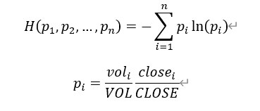voli and closei are the per-minute trading volume and per-minute closing price, while VOL and CLOSE are the total volume and total closing price over the entire time period.	High-volume trading factor: matching volume and price, Changjiang Securities
Daily post-disaster reconstruction	Optimal volatility: the square of the ratio of the standard deviation to the mean of the high-low prices over the current minute and the previous four minutes. Return-volatility ratio: the ratio of the return to the optimal volatility. Daily post-disaster reconstruction: the covariance between the return-volatility ratio and the optimal volatility.	Constructing volatility changes and “climbing peak” factor, Founder Securities
Lagged absolute return and adjusted volume correlation	Adjusted turnover: `(amount-μ)/σ` , where μ and σ are the mean and standard deviation of turnover at the same time over the previous 20 trading days. Absolute return: the absolute value of the log return. Lagged absolute return–adjusted turnover correlation: the correlation between the previous minute’s absolute return and the adjusted turnover.	High-frequency symphony of price-volume relationships, Founder Securities
Daily dazzling return	Volume surge moments: when the increase in trading volume exceeds the mean of the daily difference series plus one standard deviation. Dazzling return: the one-minute return at times of volume surge. Daily dazzling return: the average of all dazzling returns within a trading day.	Alpha from volume surge moments, Founder Securities
Daily “climbing peak”	Optimal volatility ratio: the square of the ratio of the standard deviation to the mean of high-low prices over the current minute and the previous four minutes. Return-volatility ratio: the ratio of the return to the optimal volatility. Periods of abnormally high volatility moments: when the optimal volatility exceeds its intraday mean plus one standard deviation. Daily “climbing peak”: the covariance between the return-volatility ratio series and the optimal volatility series at periods of abnormally high volatility within a trading day.	Constructing volatility changes and “climbing peak” factor, Founder Securities
Absolute return and volume correlation	Log return: the logarithm of the ratio of the current price to the price at the previous time point. Absolute return–volume correlation: the correlation between the absolute value of the log return and the trading amount.	High-frequency symphony of price–volume relationships, Founder Securities
Absolute return and lagged volume correlation	Absolute return–lagged volume correlation: the correlation between the absolute value of the log return and the trading amount at the previous time point.	High-frequency symphony of price–volume relationships, Founder Securities
Lagged absolute return and volume correlation	The correlation between the absolute value of the previous period’s log return and the trading amount.	High-frequency symphony of price–volume relationships, Founder Securities
Daily morning fog	Ordinary least squares regression with an intercept on the incremental trading volume data from minute 6 to minute 240 of each trading day: volDiff denotes the 1-minute incremental trading volume. Daily “morning fog”: the standard deviation of the t-statistics of the regression coefficients from the fifth-order incremental volume regression.	Decomposition of factors driving stock price changes and “hidden flower in the forest” factor, Founder Securities
T-distribution active proportion	T-distribution active buy amount : `amountt(ret/σ, df)` , where σ is the standard deviation of returns and df is the degrees of freedom. T-distribution active ratio*: the T-distribution active buy amount divided by the total trading amount of the day.	Active trading proportion under distribution estimation, Changjiang Securities
Confidence normal active proportion	Confidence normal distribution active buy amount: `amountN(ret/0.11.96)` , i.e., the product of the trading amount in each minute and the cumulative distribution function of the corresponding minute under the standard normal distribution. Confidence normal distribution active propotion: the confidence normal distribution active buy amount divided by the total trading amount of the day.	Active trading proportion under distribution estimation, Changjiang Securities
Naive active proportion	Naive active buy amount: `amountt(Δclose/σ, df)` , where σ is the standard deviation of the change in closing price and df is the degrees of freedom. Naive active propotion*: the active buy amount divided by the total trading amount of the day.	Active trading proportion under distribution estimation, Changjiang Securities
Uniform active proportion	Naive active buy amount: `amountt(Δclose/σ, df)` , where σ is the standard deviation of the change in closing price and df is the degrees of freedom. Naive active propotion*: the naive active buy amount divided by the total trading amount of the day.	Active trading proportion under distribution estimation, Changjiang Securities
Volume peak count	Volume peak: a time point when the trading volume is greater than the daily mean volume plus one standard deviation. Volume peak count: counts the number of records where the time difference from the previous record exceeds 1 minute.	Time-series information in high-frequency volatility, Changjiang Securities
Daily ambiguous amount proportion	Volatility: standard deviation of returns over the current and previous 4 minutes. Ambiguity: standard deviation of volatility over the current and previous 4 minutes. Foggy moment: a time when ambiguity exceeds the daily mean ambiguity. Foggy amount: average trading amount during foggy moments. Daily ambiguity amount ratio: foggy amount divided by the daily mean trading amount.	Volatility of volatility and investor ambiguity aversion, Founder Securities
Daily ambiguous count proportion	Volatility: standard deviation of returns over the current and previous 4 minutes. Ambiguity: standard deviation of volatility over the current and previous 4 minutes. Foggy moment: a time when ambiguity exceeds the daily mean ambiguity. Foggy count: average trading count during foggy moments. Daily ambiguity amount ratio: foggy amount divided by the daily mean trading amount.	Volatility of volatility and investor ambiguity aversion, Founder Securities
P-shaped volume distribution	Same-price volume: sum of all trading volumes at the same intraday minute closing price, giving the distribution of volume over price. Volume support point and support area: the price with the highest cumulative volume and its surrounding area (the smallest range where cumulative volume reaches 50% of daily total). P-shaped volume distribution: the difference between the lower bound of the volume support area and the day’s highest price.	Alpha in volume distribution, Industrial Securities
B-shaped volume distribution	Same-price volume : sum of all trading volumes at the same intraday minute closing price, giving the distribution of volume over price. Volume support point and support area: the price with the highest cumulative volume and its surrounding area (the smallest range where cumulative volume reaches 50% of daily total). B-shaped volume distribution: the difference between the upper bound of the volume support area and the day’s lowest price.	Alpha in volume distribution, Industrial Securities
Adjusted daily ambiguous price spread	Daily ambiguity price spread: daily ambiguous amount ratio minus daily ambiguous count ratio. Adjusted daily ambiguous price spread: sum all negative daily ambiguous price spreads across the cross-section as s1; divide each negative daily ambiguous price spread by the standard deviation of its past 10 days’ daily ambiguous price spreads; keep positive spreads unchanged. Scaled adjustment: sum all negative adjusted daily ambiguous price spreads across the cross-section as s2; scale each negative adjusted spread by dividing by s2 and multiplying by s1.	Ambiguity about velatlity and investor behaviot, Journal of Financial Economics
Difference between volume support zone lower bound and closing price	Same-price volume: Sum the trading volumes of minutes with the same closing price during the day to get the distribution of volume across prices. Volume support point and volume support zone: The price with the highest cumulative volume and its surrounding area (the smallest range where cumulative volume reaches 50% of the total daily volume). Difference between volume support zone lower bound and closing price: The difference between the lowest price of the volume support area and the day’s closing price.	Alpha in volume distribution, Industrial Securities
Ambiguous correlation	Volatility: The standard deviation of returns over the current and previous 4 minutes. Ambiguity: The standard deviation of volatility over the current and previous 4 minutes. Ambiguous correlation: The correlation coefficient between the ambiguous sequence and the transaction amount sequence at each time point.	Volatility of volatility and investor ambiguity aversion, Founder Securities

7.2.2 Factors Based on Level-2 Market Snapshots


Factor Name	Computation Logic and Meaning	Reference
Time-weighted average stock relative price position	Stock relative price percentile within the high-low range: 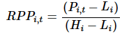Time-weighted average stock relative price position:	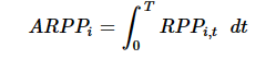Measuring intraday buying and selling pressure based on time scale, Orient Securities
High-frequency upside volatility proportion	Return : price / previous price - 1 Upside return: return > 0 High-frequency upside volatility proportion: sum of squared upward returns / sum of squared returns	High-frequency factor: decomposition of realized volatility, Guotai Haitong Securities
High-frequency downside volatility proportion	Return: price / previous price - 1 Downside return: return < 0 High-frequency downside volatility proportion: sum of squared downward returns / sum of squared returns	High-frequency factor: decomposition of realized volatility, Guotai Haitong Securities
Realized volatility	Log return series: logarithm of returns Realized volatility: square root of the sum of squared log returns	The distribution of exchange rate volatlity. Jounal of the Amencan Statistical Association 96,42-55
Realized upside volatility	Log return series: logarithm of returns Realized upside volatility: square root of sum of squared positive returns	Measuting downside risk realised semivariance, In Volatlity and Time Series Econometncs Essays in Honor of Robert F Engle Edited by T Boliersiev.J Russell and M. Watson), Oxford University Press,117-136.
Realized downside volatility	Log return series: logarithm of returns Realized downside volatility: square root of sum of squared negative returns	Measuting downside risk realised semivariance, In Volatlity and Time Series Econometncs Essays in Honor of Robert F Engle Edited by T Boliersiev.J Russell and M. Watson), Oxford University Press,117-136.
High-frequency realized skewness	Return: price / previous price - 1 High-frequency realized skewness: skewness of returns	High-frequency factor: stock return distribution characteristics, Guotai Haitong Securities
High-frequency realized kurtosis	Return: price / previous price - 1 High-frequency realized kurtosis: kurtosis of returns	High-frequency factor: stock return distribution characteristics, Guotai Haitong Securities
Upside-downside volatility asymmetry	Realized volatility: sum of squared log returns Upside realized volatility: sum of squared positive returns Downside realized volatility: sum of squared negative returns Asymmetry: (Upside realized volatility - Downside realized volatility) / Realized volatility	Measuting downside risk realised semivariance, In Volatlity and Time Series Econometncs Essays in Honor of Robert F Engle Edited by T Boliersiev.J Russell and M. Watson), Oxford University Press,117-136.
Mid-price change rate skewness	Market mid-price: average of best bid and ask Mid-price change rate: (current mid-price / previous mid-price) - 1 Skewness of mid-price change rate	High-frequency order imbalance and spread factors, China Securities
Mid-price change rate maximum	Market mid-price: average of best bid and ask Mid-price change rate: (current mid-price / previous mid-price) - 1 Maximum mid-price change rate	High-frequency order imbalance and spread factors, China Securities
Large volume realized skewness	Large volume: minute volume in the top 1/3 of the day Realized skewness for large volumes: skewness of returns for large-volume orders	Factorization method for high-frequency price-volume data, GF Securities
Large volume price-volume correlation	Large volume: minute volume in the top 1/3 of the day Correlation between price and volume for large-volume orders	Factorization method for high-frequency price-volume data, GF Securities
Realized bipower variation	Realized bipower variation: sum of products of absolute log returns and previous absolute log returns	Power and bipower variation with stochastic volatility and jumps. Journal of Financial Econometrics.2.1-48
Realized tripower variation	Tripower variation: computes the 2/3 power of products of absolute log returns at t, t-1, and t-2, then sum over the day	Power and bipower variation with stochastic volatility and jumps. Journal of Financial Econometrics.2.1-48
Daily panic	Deviation: absolute difference between the stock return and the market return (using CSI All Share Index 000985 to represent the market). Benchmark term: sum of the absolute value of the stock return, the absolute value of the market return, and 0.1. Daily panic: ratio of deviation to the benchmark term.	Significant effect, extreme return distortion decision weight, and “All is Alarm” Factor, 2022, Founder Securities. Cosemans M, Frehen R.2021, Salience theory and stock prices: Empirical evidence, Journal of Financial Economics.140(2),480-483
Volume bucket entropy	Divide intraday minute-level volumes into equal-width buckets based on max-min range; compute probability for each bucket Entropy: sum of pk * ln(pk) for all buckets, multiplied by -1	Alpha in volume distribution, Industrial Securities
Realized jump volatility	Realized tripower variation: First, compute the 2/3 power of the product of absolute log returns at each time with those at t‑1 and t‑2; then sum all these values within the trading day. Integrated volatility estimator: Realized tripower variation multiplied by the constant 1.935792405 (the 2/3‑order absolute moment of the normal distribution). Realized jump volatility: max(sum of squared log returns minus the integrated volatility estimator, 0).	Power and bipower variation with stochastic volatility and jumps. Journal of Financial Econometrics.2.1-48. New Evidence of the Marginal Predictve Content of Small and Large Jumps in the Cross-Section, Econometrics, MDPI, 8(2), 1-52.
Volume coefficient of variation	The standard deviation of the intraday trading volume series divided by its mean.	Tracking informed traders, China Merchants Securities
Upside realized jump volatility	Realized tripower variation: First, for each time point, compute the product of the absolute values of log returns at t, t-1, and t-2 raised to the 2/3 power; then sum all these values over the trading day. Integrated volatility estimator: Realized tripower variation multiplied by the constant 1.935792405 (the 2/3-order absolute moment of the normal distribution). Upside realized jump volatility: max(sum of squared log returns where returns > 0 minus half of the integrated volatility estimator, 0).	New Evidence of the Marginal Predictve Content of Small and Large Jumps in the Cross-Section, Econometrics, MDPI, 8(2), 1-52.
Downside realized jump volatility	Realized tripower variation: First, for each time point, compute the product of the absolute values of log returns at t, t-1, and t-2, raised to the 2/3 power; then sum all these values over the trading day. Integrated volatility estimator: Realized tripower variation multiplied by the constant 1.935792405 (the 2/3-order absolute moment of the normal distribution). Downside realized jump volatility: max(sum of squared log returns where returns < 0 minus half of the integrated volatility estimator, 0)	New Evidence of the Marginal Predictve Content of Small and Large Jumps in the Cross-Section, Econometrics, MDPI, 8(2), 1-52.
Smart money	Raw smart money: the ratio of the absolute value of each minute’s return to the fourth root of its trading volume. Smart money trades: select the minutes with the highest raw smart money factor until their cumulative trading volume reaches 20% of the day’s total. Volume-weighted average price (VWAP): compute the price weighted by trading volume. Smart money: the VWAP of smart money trades divided by the VWAP of all trades.	Smart money factor model v2.0, Kaiyuan Securities
Volume proportion skewness	Skewness of intraday volume proportion series	High-frequency factors IV: higher-moment factors, Changjiang Securities
Volume proportion kurtosis	Kurtosis of intraday volume proportion series	High-frequency factors IV: higher-moment factors, Changjiang Securities
Daily main force trading sentiment	Rank correlation between individual transaction amount series and close price series	High-frequency factor: characterization of main force behavior in minute-level trades, Kaiyuan Securities
Trend proportion	(Daily close - daily open) / sum of absolute price changes at each moment	Factorization method for high-frequency price-volume data, GF Securities
Upside-downside jump volatility asymmetry	Realized tripower variation: first, compute the product of the absolute values of log returns at times t, t‑1, and t‑2, raised to the 2/3 power for each minute; then sum all these values within the trading day. Integrated volatility estimate: realized tripower variation multiplied by the constant 1.935792405 (the 2/3‑order absolute moment of a normal distribution). Upside (downside) realized jump volatility : max(sum of squared log returns >0 (<0) minus half of the integrated volatility estimate, 0). Asymmetry of upside/downside jump volatility : difference between the upside and downside realized jump volatilities.	New Evidence of the Marginal Predictve Content of Small and Large Jumps in the Cross-Section, Econometrics, MDPI, 8(2), 1-52.
Maximum intraday return	Product of (1 + return) over the top 10% intraday returns	High-frequency stock selection factor taxonomy, CSC Securities
Large trade net inflow rate	Average trade amount per minute: total amount / number of trades Large trade filter: top 30% average trade amount Net inflow: sum of positive-return trades - sum of negative-return trades Net inflow rate: net inflow / total daily volume	Intraday trades insights, Guotai Haitong Securities
Large order-driven return	Average trade amount: total transaction amount per minute divided by the number of trades. Large trade filter: time points where the average trade amount ranks in the top 30%. Large-trade driven return: cumulative product of (large-trade returns + 1).	Intraday trades insights, Guotai Haitong Securities
Local reversal by trade	Sum of returns during periods where trade size (volume / number of trades) is in the 80–100% percentile	Micro-level reversal outcomes in price-volume relationships, Changjiang Securities
Average trade outflow proportion	Average trade amount with negative return / overall average trade amount	Intraday trades insights, Guotai Haitong Securities
Large upside jump volatility	Upside realized jump volatility: max⁡(difference between the sum of squared log returns where returns are greater than 0 and half of the integrated volatility estimator, 0) Discrimination threshold: where α is an empirical parameter equal to 4, Δ is the intraday sampling interval of stock returns, and IV is the integrated volatility estimator. Large upside jump volatility: min⁡(upside realized jump volatility, sum of squared log returns that exceed the discrimination threshold)	Empincal evidence on the importance of aggregaton, asymmetry and jumps for volatlty ored cnon jourral af Econometrics.187 606-621 New Evidence of the Marginal Predictve Content of Small and Large Jumps in the Cross-Section, Econometrics, MDPI, 8(2), 1-52.
Large downside jump volatility	Downside realized jump volatility: max(difference between the sum of squared log returns where returns are less than 0 and half of the integrated volatility estimator, 0) Discrimination threshold: where α is an empirical parameter equal to 4, Δ is the intraday sampling interval of stock returns, and IV is the integrated volatility estimator. Large downside jump volatility: min(downside realized jump volatility, the sum of squared log returns that are lower than the negative of the discrimination threshold)	Empincal evidence on the importance of aggregaton, asymmetry and jumps for volatlty ored cnon jourral af Econometrics.187 606-621 New Evidence of the Marginal Predictve Content of Small and Large Jumps in the Cross-Section, Econometrics, MDPI, 8(2), 1-52.
Small upside jump volatility	Upside realized jump volatility: max(difference between the sum of squared log returns where returns are greater than 0 and half of the integrated volatility estimator, 0) Discrimination threshold: where α is an empirical parameter equal to 4, Δ is the intraday sampling interval of stock returns, and IV is the integrated volatility estimator. Large upside jump volatility: min(upside realized jump volatility, sum of squared log returns that exceed the discrimination threshold) Small upside jump volatility: difference between the upside realized jump volatility and the large upside jump volatility.	Empincal evidence on the importance of aggregaton, asymmetry and jumps for volatlty ored cnon jourral af Econometrics.187 606-621 New Evidence of the Marginal Predictve Content of Small and Large Jumps in the Cross-Section, Econometrics, MDPI, 8(2), 1-52.
Small downside jump volatility	Downside realized jump volatility: max(difference between the sum of squared log returns where returns are less than 0 and half of the integrated volatility estimator, 0) Discrimination threshold: where, α is an empirical parameter equal to 4, Δ is the intraday sampling interval of stock returns, and IV is the integrated volatility estimator. Large downside jump volatility: min(downside realized jump volatility, sum of squared log returns that are lower than the negative of the discrimination threshold) Small downside jump volatility: difference between the downside realized jump volatility and the large downside jump volatility.	Empincal evidence on the importance of aggregaton, asymmetry and jumps for volatlty ored cnon jourral af Econometrics.187 606-621 New Evidence of the Marginal Predictve Content of Small and Large Jumps in the Cross-Section, Econometrics, MDPI, 8(2), 1-52.
Intraday conditional value-at-risk	Minute VWAR: the volume-weighted average of the minute return series. VaR: CVaR: VCVaR: CVaR of the intraday minute VWAR at confidence level α.	Tail characteristics of minute-level data, Founder Securities
Overnight return	Ratio of the current day’s opening price to the previous day’s closing price minus 1.	Overnight Return: the invisible Hand Behind intraday Returns, Journal of Financial Econometrics. 2.90-100
Intraday maximum drawdown	Maximum drop from peak to subsequent trough within a day	Factorization method for high-frequency price-volume data, GF Securities
Intraday volume proportion standard deviation	Standard deviation of intraday volume proportion series	High-moment high-frequency factors, Changjiang Securities
Trade-by-trade volume-return correlation	Correlation between average trade size per minute and return	Micro-level reversal outcomes in price-volume relationships, Changjiang Securities
Intraday return	Ratio of the current day’s closing price to the current day’s opening price minus 1.	Overnight Return: the invisible Hand Behind intraday Returns, Journal of Financial Econometrics. 2.90-100
Minute-level turnover variance	Variance of minute-level turnover	Hidden alpha in turnover from high-frequency perspective, Huaan Securities
Last-half-hour return	Returns from 14:30–15:00	Factorization method for high-frequency price-volume data, GF Securities
Daily order book spread	Bid-ask spread: `2(a1-b1)/(a1+b1)` , where a1 and b1 are the best ask and best bid prices. Daily bid-ask spread*: the mean of the bid-ask spread series.	Micro liquidity and volatility from a high-frequency perspective, CICC
Last-half-hour turnover proportion	Turnover proportion from 14:30–15:00	Hidden alpha in turnover from high-frequency perspective, Huaan Securities
Large upside-downside jump volatility asymmetry	Upside (downside) realized jump volatility: max⁡(difference between the sum of squared log returns where returns are greater than (or less than) 0 and half of the integrated volatility estimator, 0) Threshold: where α is an empirical parameter equal to 4, Δ is the sampling interval of intraday stock returns, and IV is the integrated volatility estimator. Large upside jump volatility: min⁡(upside realized jump volatility, sum of squared log returns exceeding the threshold) Large downside jump volatility: min⁡(downside realized jump volatility, sum of squared log returns below the negative threshold) Asymmetry of large upside and downside jumps: large upward jump volatility minus large downward jump volatility	Empincal evidence on the importance of aggregaton, asymmetry and jumps for volatlty prediction, journal of Econometrics.187 606-621 New Evidence of the Marginal Predictve Content of Small and Large Jumps in the Cross-Section, Econometrics, MDPI, 8(2), 1-52.
Small upside-downside jump volatility	Upside (downside) realized jump volatility: max⁡(difference between the sum of squared log returns where returns are greater than (or less than) 0 and half of the integrated volatility estimator, 0) Threshold: where α is an empirical parameter equal to 4, Δ is the sampling interval of intraday stock returns, and IV is the integrated volatility estimator. Large upside jump volatility: min⁡(upside realized jump volatility, sum of squared log returns exceeding the threshold) Large downside jump volatility: min⁡(downside realized jump volatility, sum of squared log returns below the negative threshold) Small upside (downside) realized jump volatility: difference between the upside (downside) realized jump volatility and the large upside (downside) realized jump volatility. Asymmetry of large upside and downside jumps: large upside jump volatility minus large downside jump volatility	Empincal evidence on the importance of aggregaton, asymmetry and jumps for volatlty prediction, journal of Econometrics.187 606-621 New Evidence of the Marginal Predictve Content of Small and Large Jumps in the Cross-Section, Econometrics, MDPI, 8(2), 1-52.
Daily price elasticity	Price elasticity: ratio of the difference between the high and low prices to the trading amount. Daily price elasticity: average of the price elasticity series over the trading day.	Micro liquidity and volatility from a high-frequency perspective, CICC
Daily average order book depth	Average order book depth: mean of the best bid and ask volumes. Daily average order book depth: mean of the order book depth series over the trading day.	Micro liquidity and volatility from a high-frequency perspective, CICC
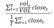
Weighted closing price ratio	where VOL refers to the total trading volume over the entire time period.	High-volume trading factor: from price-volume matching, Changjiang Securities
Structured reversal	Momentum and reversal periods: sort the time intervals by trading volume in ascending order; intervals in the bottom 10% are defined as momentum periods, and those above 10% are reversal periods. Momentum period reversal factor : Reversal period reversal factor: 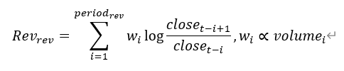Structured reversal factor: difference between the reversal period reversal factor and the momentum period momentum factor.	Structured reversal factor, Changjiang Securities
Daily effective depth	Effective depth: minimum of the best bid and ask volumes. Daily effective depth: mean of the effective depth series.	Micro liquidity and volatility from a high-frequency perspective, CICC
Minute-level turnover autocorrelation	Correlation between current minute’s turnover and previous minute’s turnover	Hidden alpha in turnover from high-frequency perspective, Huaan Securities
Last-half-hour volume proportion	Volume proportion from 14:30–15:00	Reality and illusion of high-frequency factors, Guotai Guotai Haitong Securities
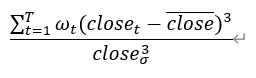
Weighted skewness	where the weight ω is the ratio of the trade volume to the total daily volume, and the denominator is the cube of the standard deviation of the closing price.	High-volume trading factor: from price-volume matching, Changjiang Securities
Synchronized informed trading probability	Trade volume buckets: divide the total trading volume into equal-volume buckets (here, each bucket has a volume of 100,000). Buy-side volume within a bucket: weighted sum of tick-by-tick trades in the bucket, with weights given by the standard normal cumulative distribution function, parameterized by the ratio of sequential increments to their standard deviation. Sell-side volume within a bucket: bucket volume minus the estimated buy-side volume. Informed trading probability synchronized with volume: the sum of absolute differences between buy-side and sell-side volumes, divided by the total trading volume.	Flow toxicity and liquidity in a high frequency world, Review of Financial Studies, 25(5),457-1493.

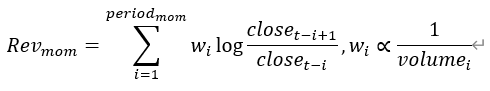
7.2.3 Factors Based on Tick-by-Tick Orders


Factor Name	Computation logic and meaning	Reference
Post-open buy intention intensity	Net change in buy orders: increase in buy orders minus increase in sell orders (tick-by-tick orders). Net aggressive buy volume: aggressive buy volume minus aggressive sell volume. Buy intention: sum of net aggressive buy volume and net change in buy orders. Post-open buy intention strength: mean of the buying intention series during the post-open period (9:30–10:00) divided by its standard deviation.	Low-frequency applications of high-frequency data based on intuitive logic and machine learning, Guotai Haitong Securities
Post-open net buy order increase proportion	Net change in buy orders: increase in buy orders minus increase in sell orders. Post-open net buy order proportion: total net change in buy orders during the post-open period (9:30–10:00) divided by the total trading volume in the same period.	Capturing investor trading intentions, Guotai Haitong Securities; Reality and illusions of high-frequency factors, Guotai Haitong Securities
Post-open buy intention proportion	Net change in buy orders: increase in buy orders minus increase in sell orders (tick-by-tick orders). Net active buy volume: active buy volume minus active sell volume. Buy intention: sum of net active buy volume and net change in buy orders. Post-open buy intention strength: sum of buy intention during the post-open period (9:30–10:00) divided by the total trading volume in the same period.	Low-frequency applications of high-frequency data based on intuitive logic and machine learning, Guotai Haitong Securities

7.2.4 Factors Based on Tick-by-Tick Trades


Factor Name	Computation Logic and Meaning	Reference
Sell rebound deviation	(Sum of average trade prices of sell orders below the day's closing price / closing price) − 1	Regret-aversion factors based on tick-by-tick trades, SinolinkSecurities
Large buy order proportion	Large order selection: After logarithmic adjustment of trade volume, select trades where the volume is greater than the mean plus 1 standard deviation. Large order buy proportion: Total value of large buy orders divided by total trading value.	Fine-tuned large Order processing and large order factor reconstruction, Guotai Haitong Securities; Alpha in buy/sell orders, Guotai Haitong Securities
Buy order concentration	Sum of squared buy order amounts divided by square of total buy amount	Alpha in buy/sell orders, Guotai Haitong Securities
Sell order concentration	Sum of squared sell order amounts divided by square of total sell amount	Alpha in buy/sell orders, Guotai Haitong Securities
Post-open large net buy proportion	Large order selection: After logarithmic adjustment of trade volume, select trades where the volume is greater than the mean plus 1 standard deviation. Post-open net large buy proportion: difference between large buy order value and large sell order value during the post-open period (9:30–10:00) divided by total trading value.	Alpha in buy/sell orders, Guotai Haitong Securities; Fine-tuned large order processing and large order factor reconstruction, Guotai Haitong Securities
Intraday active buy proportion	Active buy trade value: sum of trade amounts marked as “Buy” in the tick-by-tick data, excluding trades that occur during price limit minutes. Intraday active buy ratio: Active buy trade value divided by the total trading value of the day.	Stock selection factor based on active buy behavior, Guotai Haitong Securities
Large buy order intensity	Large order selection: orders whose log-adjusted volume is greater than the mean plus one standard deviation. Large buy order intensity: intraday mean of large buy order trade values divided by their intraday standard deviation.	Fine-tuned large order processing and large order factor reconstruction, Guotai Haitong Securities
Post-open net active buy proportion	Net aggressive buy volume: difference between aggressive buy and sell trade values, excluding trades during price limit minutes. Post-open net buy proportion: ratio of net aggressive buy volume to total trade value during the post-open period (9:30–10:00).	Stock selection factor based on active buy behavior, Guotai Haitong Securities; reality and illusions of high-frequency factors, Guotai Haitong Securities
Intraday active buy intensity	Aggressive buy trade value: value of trades marked as “Buy”, excluding trades during price-limit minutes. Intraday active buy strength: ratio of the mean to the standard deviation of active buy trade values.	Stock selection factor based on active buy behavior, Guotai Haitong Securities
Post-open net active buy intensity	Net active buy trade value: difference between active buy and sell trade values, excluding trades during price-limit minutes. Post-open net buy strength: ratio of the mean to the standard deviation of net active buy trade values during the post-open period (9:30–10:00).	Stock selection factor based on active buy behavior, Guotai Haitong Securities; reality and illusions of High-frequency factors, Guotai Haitong Securities
Sell-order illiquidity	A linear regression with returns as the dependent variable and main sell and buy trade values as independent variables, taking the regression coefficient of the main sell trade value.	Sell-order liquidity and the cross section of expected stock retutns, Journat of Financial Economeics 105(3) 523-541 ; Batch Testing of Technical Alpha Factors, Orient Securities
Buy-order illiquidity	A linear regression with returns as the dependent variable and main sell and buy trade values as independent variables, taking the regression coefficient of the active buy trade value.	Sell-order liquidity and the cross section of expected stock retutns, Journat of Financial Economeics 105(3) 523-541 ; Batch Testing of Technical Alpha Factors, Orient Securities
Sell rebound proportion	The ratio of the total volume of all sell orders with prices below the closing price to the total trading volume.	Regret-aversion factors based on tick-by-tick trades, Sinolink Securities
Normal large buy proportion(excluding mega orders)	Large order selection: orders whose transaction amounts are above the 70th percentile. Extra-large order selection: orders whose transaction amount exceeds 1% of the total daily trading volume. Proportion of ordinary large buy orders excluding extra-large orders: the total amount of large buy orders after excluding extra-large orders divided by the total amount of all large orders.	Impact of mega orders on large order factors, Orient Securities
Mega buy proportion	Mega order selection: orders whose transaction amount exceeds 1% of the total daily trading volume. Mega buy ratio: total amount of mega buy orders divided by the total amount of all mega orders.	Impact of mega orders on large order factors, Orient Securities
Small buy order aggressiveness	Small order selection: After log-adjusting the trade volume, select orders with volume below the mean. Small buy order aggressiveness: proportion of small buy orders executed actively (active buys) relative to the total small buy order volume.	Hidden information in buy/sell order activity, Haitong Securities
Large order price change excluding mega orders	Large order selection: select orders whose trade amount is above the 70th percentile. Mega order selection: select orders whose trade amount accounts for more than 1% of the day’s total trading volume. Log price change: difference between the logarithm of the current trade price and the logarithm of the previous trade price. Large order return excluding mega order impact: the cumulative log price changes of large main trades after excluding mega orders.	Impact of mega orders on large order factors, Orient Securities
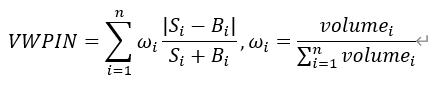
Informed trading probability weighted by physical time volume	where Si and Bi are the number of sell orders and buy orders in the i-th trading interval, respectively.	Informed trading probability and risk pricing – comparison of different PIN measures, Management Science Journal 23(1), 33–46
Mega order price change	Large order selection: orders whose trade amount accounts for more than 1% of the total daily turnover. Log price change: difference between the logarithm of the current trade price and the previous trade price. Large order price change: cumulative log price change of large active orders.	Impact of mega orders on large order factors, Orient Securities
Buy floating loss proportion	Sum of buy order volumes with trade prices above the day’s closing price, divided by the total daily trading volume.	Regret-aversion factors based on tick-by-tick trades, Sinolink Securities
Buy floating loss deviation	Average executed price of buy orders above daily close / close – 1	Regret-aversion factors based on tick-by-tick trades, Sinolink Securities
Post-open large net buy intensity	Large order selection: trades whose log-adjusted volume is greater than the mean plus one standard deviation. Post-open large order net buy intensity: intraday mean of the difference between large buy and large sell order amounts during the post-opening period (9:30–10:00) divided by its standard deviation.	Fine-tuned large order processing and large order factor reconstruction, Haitong Securities
Large volume order execution proportion	Large-volume order selection: count the traded volume by order ID and select the top 5% of orders by volume. Large-volume order trade proportion: the total traded volume of large-volume orders divided by the total traded volume for the entire day.
Large volume trade execution proportion	Large-volume trade selection: from the tick-by-tick transaction data, select the top 5% of orders by traded volume. Large-volume trade proportion: total traded volume of these large-volume trades divided by the total traded volume for the entire day.

7.3 Full Code for Database Setup, Factor Computation, and Factor Storage

general_factor_computation_template.dos