Probability and Statistical Analysis
DolphinDB provides a comprehensive suite of built-in statistical functions designed for efficient probability and statistical analysis. With these functions, users can effortlessly perform probability and statistical analysis such as probability districution, random number generation, regression analysis, and hypothesis testing. These capabilities enable efficient data modeling and analysis, supporting critical tasks like financial risk management, investment strategies, and IoT insights.
1. Probability and Statistics
DolphinDB provides comprehensive support for univariate and multivariate probability
functions. This section covers the implementation and usage of complex univariate
statistical measures such as mad, kurtosis and
skew, as well as important multivariate metrics like covariance
and correlation coefficients.
1.1 Univariate Statistics
Univariate statistics measures a single variable individually, focusing on patterns like central tendency and dispersion. The univariate statistics functions supported by DolphinDB are listed below. Note that DolphinDB ignores null values when calculating univariate statistical features.
| Statistical Feature | Function |
|---|---|
| Minimum Value | min |
| Maximum Value | max |
| Mean | mean,
avg |
| Unbiased Sample Variance | var |
| Population Variance | varp |
| Unbiased Sample Standard Deviation | std |
| Population Standard Deviation | stdp |
| Unbiased Standard Error of Mean | sem |
| Median | med |
| Percentile | percentile |
| Mean Absolute Deviation | mad(X, useMedian=false) |
| Median Absolute Deviation | mad(X, useMedian=true) |
| Kurtosis | kurtosis |
| Skewness | skew |
| Autocorrelation | acf,
autocor |
Common statistical features such as min, max, mean, avg, std, and percentile can
be obtained using the summary function. The following is a
simple example of preliminary exploratory data analysis on three years of data
for three stocks using summary.
n=2022
data=1..2022
value=take(1..3,n)
name=take(`APPLE`IBM`INTEL,n)
t=table(data,value,name);
res = summary(t, precision=0.001);
res

/*Output
	name	min	max	nonNullCount	count	avg	std	percentile
0	data	1.00	2022.00	2022	2022	1011.50	583.85	[506.25, 1011.50, 1,516.75]
1	value	1.00	3.00	2,022	2,022	2.000	0.8166985591	[1.00, 2.00, 3.00]
*/
The following sections will focus on more complex univariate statistical features such as mad, kurtosis, and skewness.
1.1.1 Mean Absolute Deviation (MAD)
The mean absolute deviation (MAD) serves as a reliable measure of dispersion,
reflecting the spread or variability of data points around the mean.
However, when used in statistical inference, its statistical properties are
inferior to the standard deviation. The mad function by
default calculates the mean absolute deviation, and the formula is as
follows:

The following results show that the calculations from DolphinDB and Python Numpy are consistent up to 8 decimal places.
import time
import numpy as np
import dolphindb as ddb

def calculate_mad(data):
    med = np.median(data)
    abs_diffs = np.abs(data - med)
    return np.median(abs_diffs)

# Set random seed to ensure reproducibility
np.random.seed(42)

data = np.random.randint(1, 101, size=10000)

# Calculate MAD using Python Numpy
result1 = calculate_mad(data)
print(f"MAD value using Python Numpy: {result1:.8f}")

# Calculate MAD using DolphinDB
s = ddb.session()
s.connect("localhost", 7271)
result2 = s.run("mad{,true}", data)
print(f"MAD value using DolphinDB: {result2:.8f}")

# Data validation
abs_diff = abs(result1 - result2)
if abs_diff < 1e-8:
    print("MAD calculation results are consistent up to 8 decimal places.")
else:
    print(f"MAD calculation results differ by: {abs_diff:.8f}")

s.close()

/* output
MAD value using Python Numpy: 25.00000000
MAD value using DolphinDB: 25.00000000
MAD calculation results are consistent up to 8 decimal places.
*/
1.1.2 Median Absolute Deviation (MAD)
The median absolute deviation (MAD) is a robust measure of statistical
dispersion, providing an alternative to the mean absolute deviation that is
less influenced by extreme outliers. It improves upon the traditional
absolute deviation by using the median as a reference. To calculate the
median absolute deviation, the mad function must specify
useMedian=true. The formula for calculating MAD is as
follows:

The following results show that the calculations from DolphinDB and Python Numpy are consistent up to 8 decimal places.
import time
import numpy as np
import dolphindb as ddb

def calculate_mad(data):
    med = np.median(data)
    abs_diffs = np.abs(data - med)
    return np.median(abs_diffs)

# Set random seed to ensure reproducibility
np.random.seed(42)

data = np.random.randint(1, 101, size=10000)

# Calculate MAD using Python Numpy
result1 = calculate_mad(data)
print(f"MAD value using Python Numpy: {result1:.8f}")

# Calculate MAD using DolphinDB
s = ddb.session()
s.connect("localhost", 7271)
result2 = s.run("mad{,true}", data)
print(f"MAD value using DolphinDB: {result2:.8f}")

# Data validation
abs_diff = abs(result1 - result2)
if abs_diff < 1e-8:
    print("MAD calculation results are consistent up to 8 decimal places.")
else:
    print(f"MAD calculation results differ by: {abs_diff:.8f}")

s.close()

/* output
MAD value using Python Numpy: 25.00000000
MAD value using DolphinDB: 25.00000000
MAD calculation results are consistent up to 8 decimal places.
*/
MAD can be effectively used to detect outliers. The process typically involves the following steps:
- Use the
medfunction to obtain the median of the dataset to serve as the central reference. - For each data point, use the
madfunction to calculate the median absolute deviation. - Set an outlier threshold, usually as a multiple of MAD.

- Detect and mark outliers for further analysis.

The following example demonstrates how to use median absolute deviation for identifying and handling outliers via winsorization:
/* Identifying outliers based on MAD
   Input : original data
   Output : indexes of outliers
 */
def winsorized(X){
    // calculate the median and mean absolute deviation
    medianX = median(X)
    madX = mad(X, true)
    sigma = 1.4826*madX
    // calculate the lower and upper limits
    lowerLimit = medianX - 3*sigma
    upperLimit = medianX + 3*sigma
    // winsorize the data
    indexes = 0..(X.size()-1)
    return indexes.at(X < lowerLimit || X > upperLimit)
}
X = [-5.8, 2, 3, 4, 5, 6, 7, 8, 9, 18]
winsorized(X)
// output: [0, 9]
1.1.3 Skewness
Skewness measures the asymmetry of the probability distribution of a real-valued random variable about its mean. The skewness value can be:
- Positive (right-skewed): The tail is more pronounced on the right side than on the left.
- Negative (left-skewed): The tail is more pronounced on the left rather than the right.
- Zero: Values are relatively evenly distributed around the mean.
Skewness can be computed using the skew function when the
sample size n≥3. Let x̄ be the sample mean, s be the sample standard
deviation, and m3 be the third central moment of the sample. The
formula for sample skewness is:

Note that the skewness computed in Python and Excel differs from the above. These tools calculate the Fisher-Pearson standardized moment G1, which adjusts the sample skewness for bias. The formula is:

To compute the Fisher-Pearson standardized moment G1 in DolphinDB, you can use the following script. The results show that the calculations from DolphinDB and Python pandas are consistent up to 8 decimal places.
import pandas as pd
import numpy as np
import dolphindb as ddb

# Set random seed to ensure reproducibility
np.random.seed(42)
data = np.random.normal(0, 1, 1000)

# Calculate Fisher-Pearson skewness using Python pandas
result1 = pd.Series(data).skew()
print(f"skewness using Python pandas: {result1:.8f}")

# Calculate Fisher-Pearson skewness using DolphinDB
session = ddb.session()
session.connect("localhost", 7271)
session.upload({"n":len(data),"x":data})
result2 = session.run("sqrt(n*(n-1))\(n-2)*skew(x)")
print(f"skewness using DolphinDB: {result2:.8f}")

# Data validation
abs_diff = abs(result1 - result2)
if abs_diff < 1e-8:
    print("Skewness calculation results are consistent up to 8 decimal places.")
else:
    print(f"Skewness calculation results differ by: {abs_diff:.8f}")

session.close()

/* output
Skewness value using Python pandas: 0.11697637
Skewness value using DolphinDB: 0.11697637
Skewness calculation results are consistent up to 8 decimal places.
*/
1.1.4 Kurtosis
Kurtosis refers to a descriptive statistic used to measure how data disperse between the center and tails of a distribution. A higher kurtosis indicates that the variance is primarily driven by extreme values (either larger or smaller than the mean) that occur less frequently.
In DolphinDB, the kurtosis is calculated as an estimate of the fourth central moment. Subtracting 3 from the result yields a value that aligns with Python’s kurtosis calculation.
- By default, biased=true is used to calculate the sample kurtosis,
which results in a biased estimate. Let the sample mean be denoted by
x̄, the sample standard deviation by s, and the fourth central moment by
m4. The formula for sample kurtosis is as
follows:

- If biased=false is specified, the calculation is for the
population kurtosis, which provides an unbiased estimate for a normal
distribution. The formula is as follows:

Since the kurt function in Python pandas calculates the
unique symmetric unbiased estimator of the fourth cumulant (i.e., excess
kurtosis), the results from DolphinDB's kurtosis function
match those of pandas after subtracting 3, as shown in the following
script.
import pandas as pd
import Numpy as np
import dolphindb as ddb

# Set random seed to ensure reproducibility
np.random.seed(42)
data = np.random.normal(0, 1, 1000)

# Calculate kurtosis using Python pandas
result1 = pd.Series(data).kurt()
print(f"Kurtosis (Pandas): {kurt_pandas:.8f}")

# Calculate kurtosis using DolphinDB
session = ddb.session()
session.connect("localhost", 7271)
result2 = session.run("kurtosis{,false}",data)-3
print(f"Kurtosis (DolphinDB): {kurt_dolphindb:.8f}")

# Data validation
abs_diff = abs(result1 - result2)
if abs_diff < 1e-8:
    print("Kurtosis calculation results are consistent up to 8 decimal places.")
else:
    print(f"Kurtosis calculation results differ by: {abs_diff:.8f}")

session.close()

/* output
Kurtosis (Pandas): 0.07256220
Adjusted Kurtosis (DolphinDB): 0.07256220
Kurtosis calculation results are consistent up to 8 decimal places.
*/
1.2 Multivariate Statistics
Multivariate statistics refers to the analysis of relationships between multiple variables, including the calculation of statistical features such as covariance and correlation coefficients. These measures help users understand the linear relationships and the degree of mutual influence between variables. DolphinDB provides a variety of functions to support the statistical analysis of multivariate features, which are listed below. This section will introduce the implementation and usage of these functions in detail.
| Statistical Feature | Function |
|---|---|
| Covariance | covar |
| Covariance Matrix | covarMatrix |
| Pearson Correlation Coefficient | corr |
| Pearson Correlation Matrix | corrMatrix |
| Spearman’s Rank Correlation Coefficient | spearmanr |
| Kendall Correlation Coefficient | kendall |
| Weighted Covariance | wcovar |
1.2.1 Covariance and Covariance Matrix
Covariance measures the joint variability of two random variables. A
covariance matrix is a square matrix giving the covariance between each pair
of elements across all dimensions. In DolphinDB, the covar
function calculates the sample covariance between two vectors using the
following formula:

For multi-dimensional data, DolphinDB provides the
covarMatrix function to compute the covariance matrix,
using the formula:

The following example demonstrates how to construct a risk matrix in DolphinDB:
returns_a = [0.01, 0.02, -0.03, 0.01, 0.02]
returns_b = [-0.02, 0.01, 0.03, -0.02, -0.01]
returns_c = [0.03, -0.01, -0.02, 0.02, 0.01]
m = matrix(returns_a, returns_b, returns_c).rename!(`a`b`c)
covariance_matrix = covarMatrix(m)
/* output:
	a	b	c
a	0.0004300000	-0.0003100000	0.0002300000
b	-0.0003100000	0.0004700000	-0.0004350000
c	0.0002300000	-0.0004350000	0.0004300000
*/
1.2.2 Pearson Correlation Coefficient and Correlation Matrix
Pearson correlation coefficient measures linear correlation between two
variables. In DolphinDB, the correlation coefficient can be calculated using
the corr function, using the formula:

For multi-dimensional data, DolphinDB provides the
corrMatrix function to compute the correlation matrix,
using the formula:

The Pearson correlation coefficient between a market index and individual stock returns shows the correlation between the stock and the overall market. For example:
// Market index data
market_index = [100, 110, 120, 130, 140]
// Individual stock return data
stock_returns = [0.01, 0.02, 0.03, -0.01, 0.02]
corr(market_index, stock_returns)
// Output: -0.1042572070
In portfolio optimization, correlation matrix can help reveal the correlation between different assets. This allows investors to select assets with low correlations in the portfolio for better diversification. For example, select assets with low correlations to others:
setRandomSeed(42)
m = rand(10.0, 100)$10:10
c= corrMatrix(m)
result = table(1..10 as stock_code,
               c[c<0.5].abs().sum() as corr_sum).sortBy!(`corr_sum)
result
/* Output
	stock_code	corr_sum
0	8	1.6943835693
1	2	1.9124975741
2	6	1.9699810000
3	10	1.9706433980
4	4	1.9955912515
5	1	2.0791768735
6	9	2.2377748096
7	5	2.2757034717
8	7	2.8368851661
9	3	3.0716024528
*/
1.2.3 Spearman’s Rank Correlation Coefficient
The Spearman’s rank correlation coefficient is a non-parametric measure of
rank correlation, essentially the Pearson correlation coefficient applied to
ranked variables. In DolphinDB, it can be computed using the
spearmanr function, using the formula:

In quantitative trading, the Information Coefficient (IC) measures the
correlation between predicted and actual future returns, often used to
evaluate the forecasting and stock-picking abilities. The
spearmanr function is commonly used to calculate the
Rank IC values. The result of spearmanr is consistent with
the rank-based correlation computed using corr.
setRandomSeed(123)
predicted_returns = rand(1.0, 100)
actual_returns = rand(1.0, 100)
r1 = spearmanr(predicted_returns, actual_returns)
r2 = corr(rank(predicted_returns) + 1, rank(actual_returns) + 1)
eqObj(r1, r2)
// output: true
2. Probability Distributions
DolphinDB supports an extensive range of discrete and continuous probability distributions, offering functions for probability density, cumulative density, and random number generation. This section highlights the application of DolphinDB in discrete distributions, including Poisson and Binomial, as well as continuous distributions such as Normal, t, F, and Chi-square distributions.
| Distribution | Cumulative Density Function (CDF) | Inverse CDF | Random Number Generator |
|---|---|---|---|
| Normal Distribution | cdfNormal |
invNormal |
randNormal |
| Binomial Distribution | cdfBinomial |
invBinomial |
randBinomial |
| Poisson Distribution | cdfPoisson |
invPoisson |
randPoisson |
| Zipf Distribution | cdfZipf |
||
| t Distribution | cdfStudent |
invStudent |
randStudent |
| Chi-square Distribution | cdfChiSquare |
invChiSquare |
randChiSquare |
| F Distribution | cdfF |
invF |
randF |
| Exponential Distribution | cdfExp |
invExp |
randExp |
| Gamma Distribution | cdfGamma |
invGamma |
randGamma |
| Logistic Distribution | cdfLogistic |
invLogistic |
randLogistic |
| Uniform Distribution | cdfUniform |
invUniform |
randUniform |
| Weibull Distribution | cdfWeibull |
invWeibull |
randWeibull |
| Kolmogorov Distribution | cdfKolmogorov |
||
| Beta Distribution | cdfBeta |
invBeta |
randBeta |
2.1 Discrete Distributions
2.1.1 Bernoulli Distribution (0-1 Distribution)
Bernoulli distribution (0-1 distribution) is a basic univariate distribution and serves as the basis for the Binomial distribution. Suppose an investment strategy generates daily returns as a binary random variable, which could either be a positive return (1) or a negative return (0), with no cases of no gain or loss. This aligns with the following description:

The probability of positive returns pwin determines all the
characteristics of the Bernoulli distribution. For example, if
pwin=0.5, the probability mass function (PMF) of the 0-1
distribution can be calculated using the pmfBernoulli
function in DolphinDB.
def pmfBernoulli(p){
   cdf = cdfBinomial(1, p, [0,1])
   pmf =table([0,1] as X,cdf -prev(cdf).nullFill(0) as P).sortBy!(`X)
   return pmf
}
p = 0.5
pmfBernoulli(p)
/* Output
	X	P
0	0	0.50
1	1	0.50
*/
In DolphinDB, once the probability pwin of a 0-1 event and the
number of trials N are defined, the randBernoulli function
can be used to simulate Bernoulli trials. For instance, assume each positive
return corresponds to a logarithmic return of 10%, and each negative return
corresponds to -10%. After running N trials according to the strategy, the
total return can be calculated by summing the logarithmic returns. The
following example shows that the return after 10 investment periods is
22%.
setRandomSeed(40393)
def randBernoulli(p, n){
   return randBinomial(1, p, n)
}
x = randBernoulli(0.5, 10)
// Suppose each period's logarithmic return is fixed at 0.1
log_return = 0.1
exp(sum(log_return * iif(x == 0, -1, x))) - 1
// Output: 0.2214
2.1.2 Binomial Distribution
Evaluating the probability and frequency of positive returns can be modeled using the Binomial distribution. A random variable X that follows a Binomial distribution with parameters p (probability of a 0-1 event) and n (number of trials) is denoted as X∈B (n, p) . The probability mass function (PMF) for X=k is expressed as:

In DolphinDB, the pmfBinomial function can be used to
compute the PMF of a Binomial distribution. For example, the following
result shows that after 10 trials, the probability of achieving exactly 5
positive returns is approximately 24.61%.
def pmfBinomial(trials, p){
    X = 0..trials
    cdf = cdfBinomial(trials, p, X)
    return table(X, cdf - prev(cdf).nullFill(0) as P).sortBy!(`X)
}
pmfBinomial(10, 0.5)

/* output:
X  P
-- -----------------
0  0.0009765625
1  0.009765625
2  0.0439453125
3  0.1171875
4  0.205078125
5  0.246093749999999
6  0.205078125
7  0.1171875
8  0.0439453125
9  0.009765625
10 0.0009765625
*/
Using the pmfBinomial function, we can visualize the
Binomial distribution under varying probabilities p and trial numbers n.
Note that only integer values of X are valid.
plot([pmfBinomial(20,0.5)["P"] <- take(double(),20) as "p=0.5,n=20",
      pmfBinomial(20,0.7)["P"] <- take(double(),20) as "p=0.7,n=20",
      pmfBinomial(40,0.5)["P"] as "p=0.5,n=40"],0..40,"Binomial Distributions")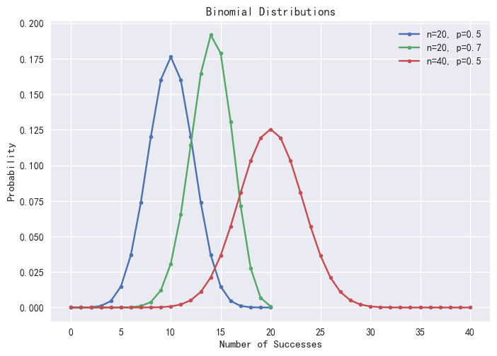
2.1.3 Poisson Distribution
The Poisson distribution is a statistical model used to describe the occurrence of events over a continuous space or time interval. It is closely related to the Binomial distribution but differs in focus. While the Binomial distribution models the number of successes in a fixed number of trials, the Poisson distribution focuses on the number of discrete events occurring within a continuous interval. The probability mass function (PMF) of the Poisson distribution is defined as:

In DolphinDB, the pmfPoisson function can be used to compute
the PMF values of a Poisson distribution. Note that only integer values of X
are valid, and visual grouping is often done with lines connecting discrete
points.
def pmfPoisson(mean, upper=20){
   x = 0..upper
   cdf =cdfPoisson(mean, x)
   pmf =table(x as X, cdf - prev(cdf).nullFill(0) as P).sortBy!(`X)
   return pmf
}
plot([pmfPoisson(1)["P"] as "λ=1",
      pmfPoisson(4)["P"] as "λ=4",
      pmfPoisson(10)["P"] as "λ=10"],
      0..20,"Poisson Distributions")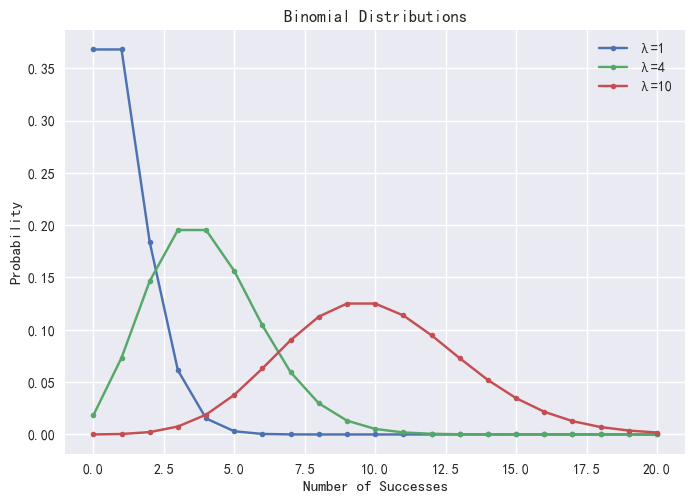
2.2 Normal Distribution
The normal distribution (Gaussian distribution) is a probability distribution that is symmetric about the mean, showing that data near the mean are more frequent in occurrence than data far from the mean. The Central Limit Theorem states that the mean of a sufficiently large sample from any distribution approaches a normal distribution. Mathematically, a normal distribution is characterized by its mean μ and standard deviation σ.

In DolphinDB, the norm function generates data that follows
X∈N (μ, σ), returning a vector or matrix of the
specified dimensions. For example:
setRandomSeed(123)
X = norm(2.0, 0.1, 1000);
print mean X // output: 2.003
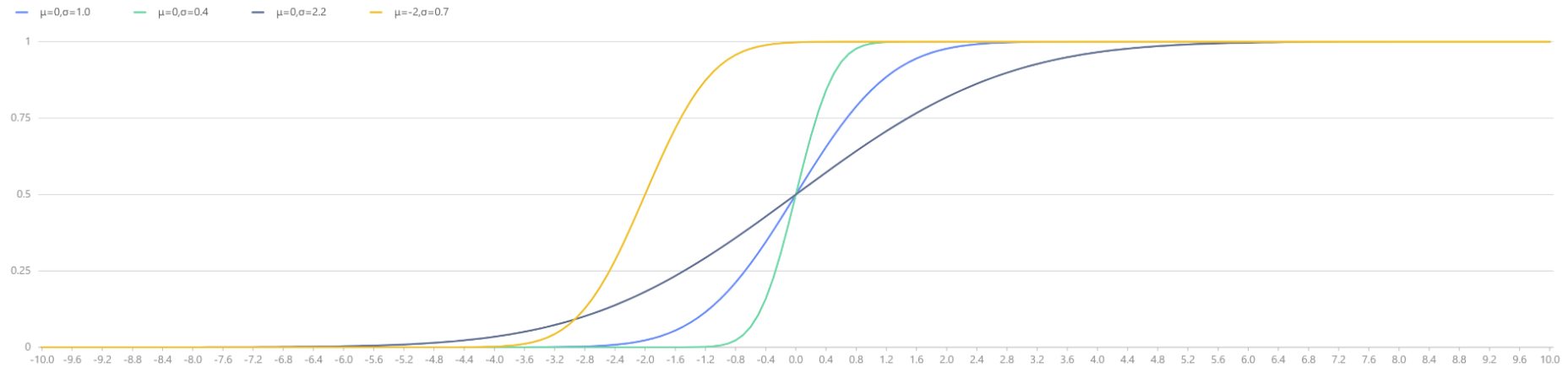
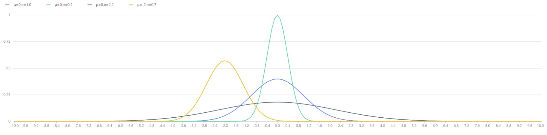
print std X // output: 0.102Using the pdfNormal and cdfNormal functions, we
can plot the Probability Density Function (PDF) and Cumulative Density Function
(CDF) for various values of μ and σ:
x = 0.1*(-100..100)
plot([pdfNormal(0,1.0,x) as "μ=0,σ=1.0", pdfNormal(0,0.4,x) as "μ=0,σ=0.4",
      pdfNormal(0,2.2,x) as "μ=0,σ=2.2", pdfNormal(-2,0.7,x) as "μ=-2,σ=0.7"],
      x, "Normal Distributions with Different Parameters μ and σ")
plot([cdfNormal(0,1.0,x) as "μ=0,σ=1.0", cdfNormal(0,0.4,x) as "μ=0,σ=0.4",
      cdfNormal(0,2.2,x) as "μ=0,σ=2.2", cdfNormal(-2,0.7,x) as "μ=-2,σ=0.7"],
      x, "Normal Distributions with Different Parameters μ and σ")
|
|
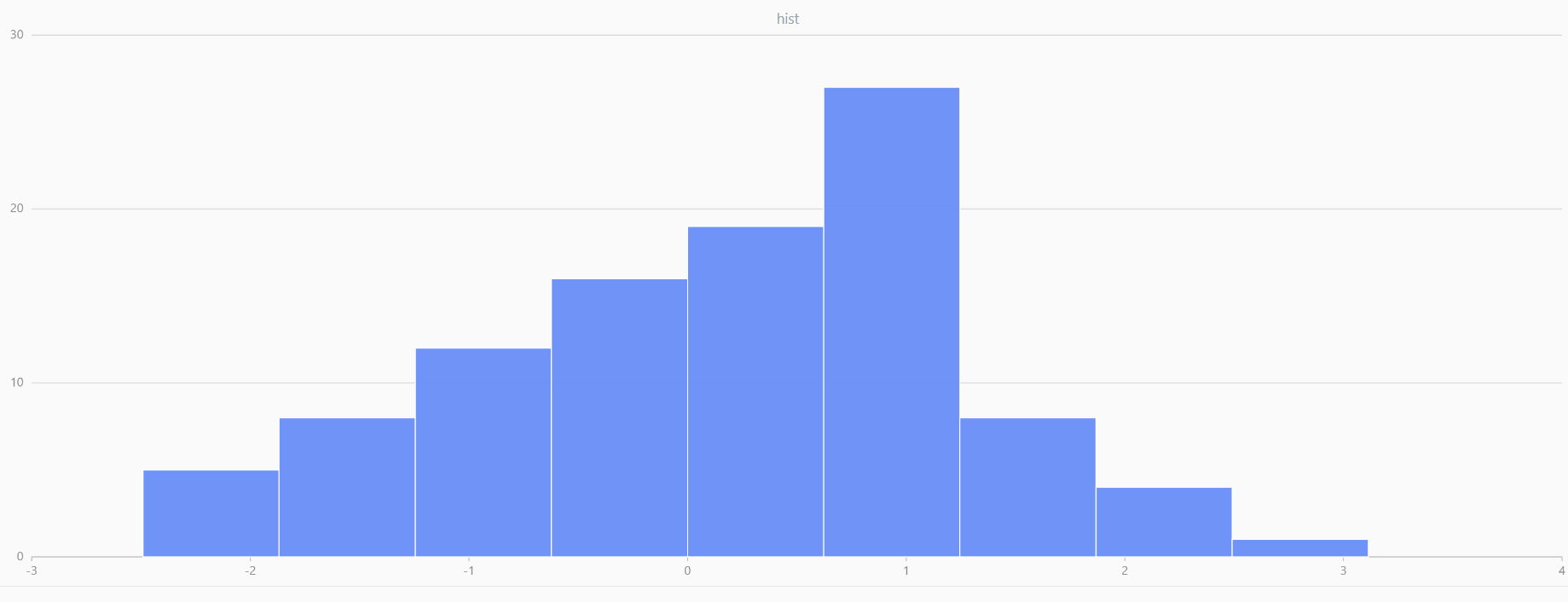
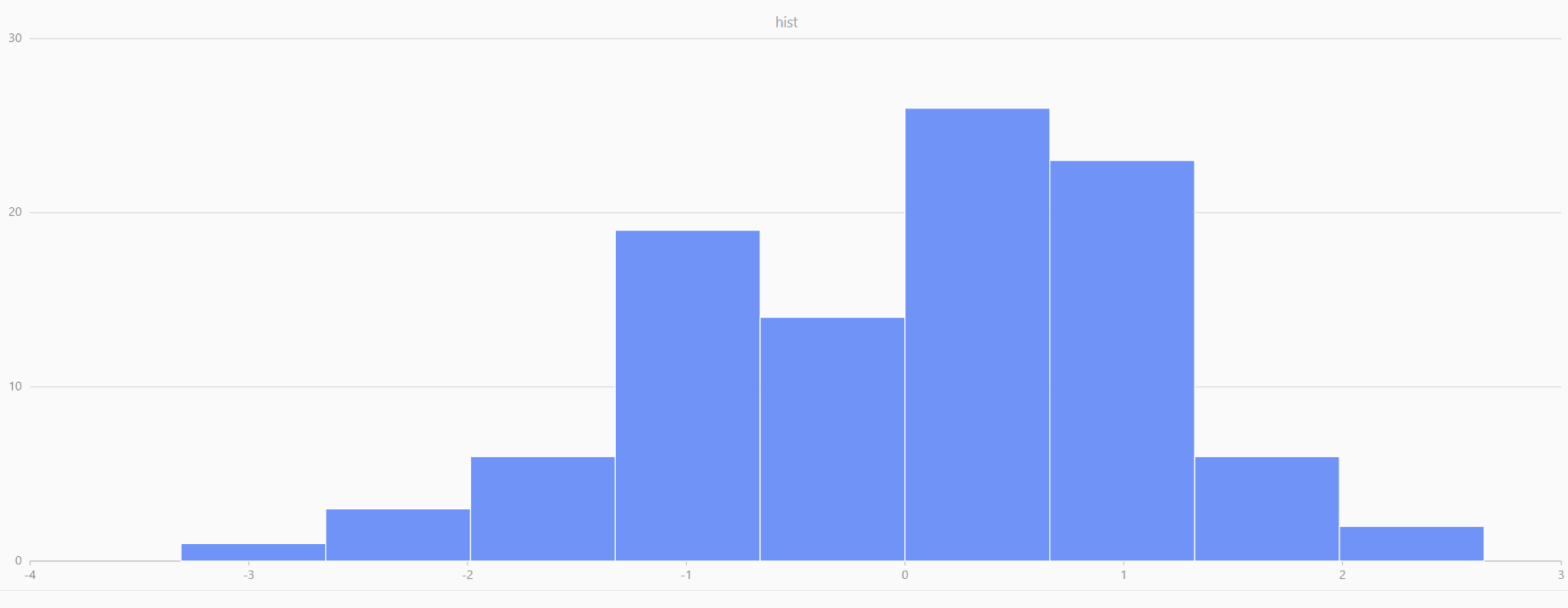
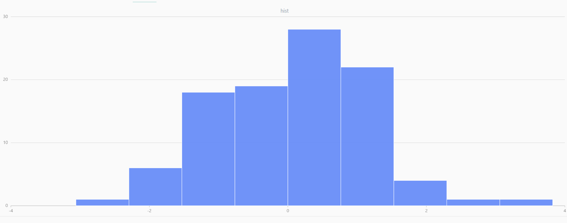
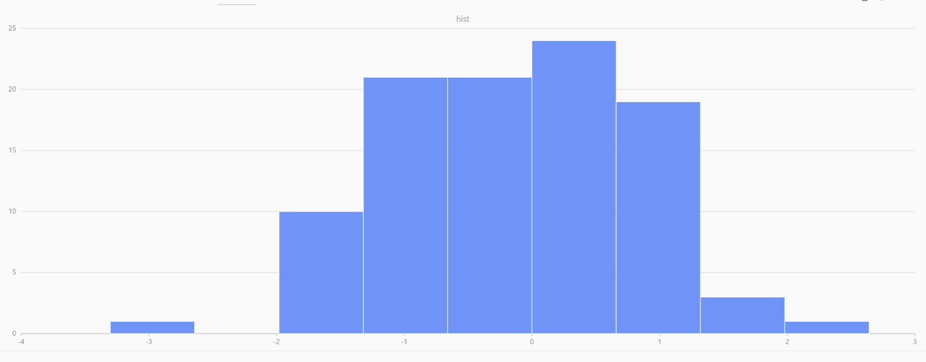
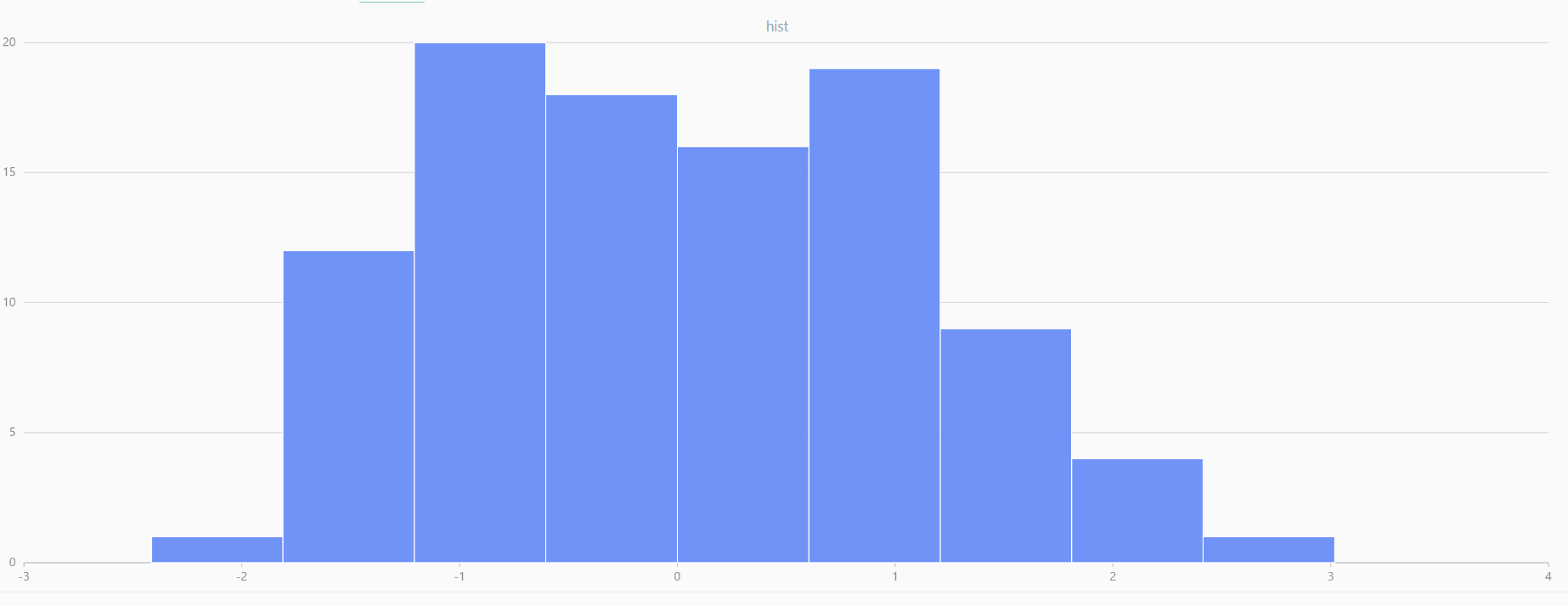
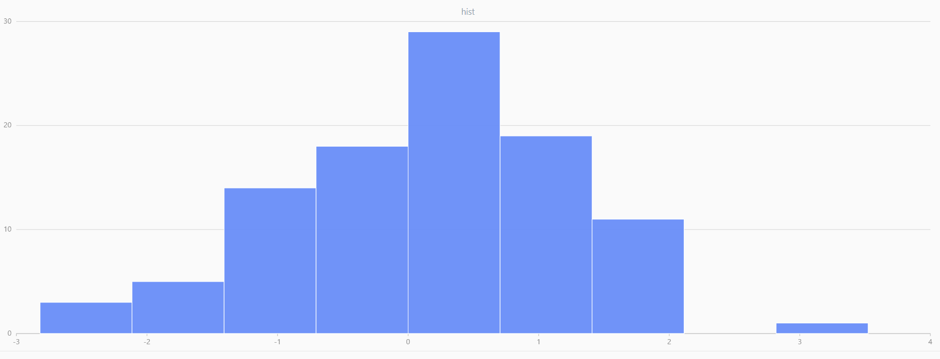
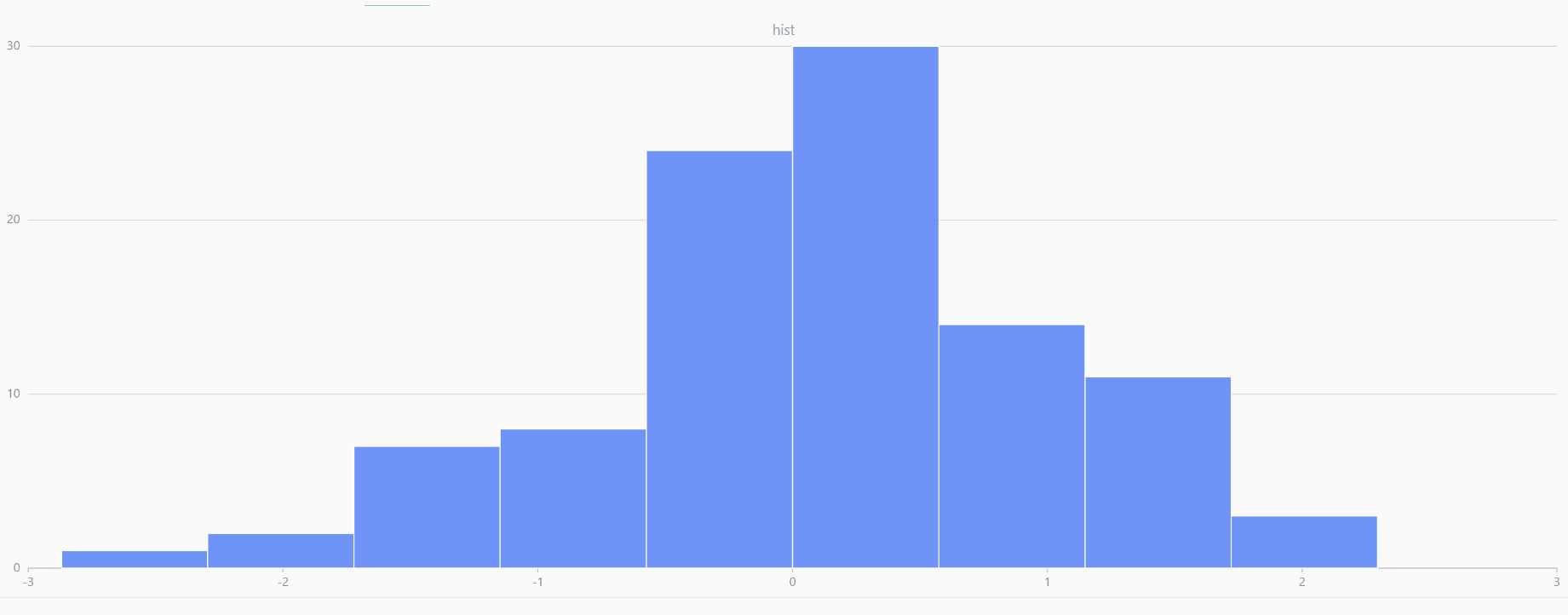
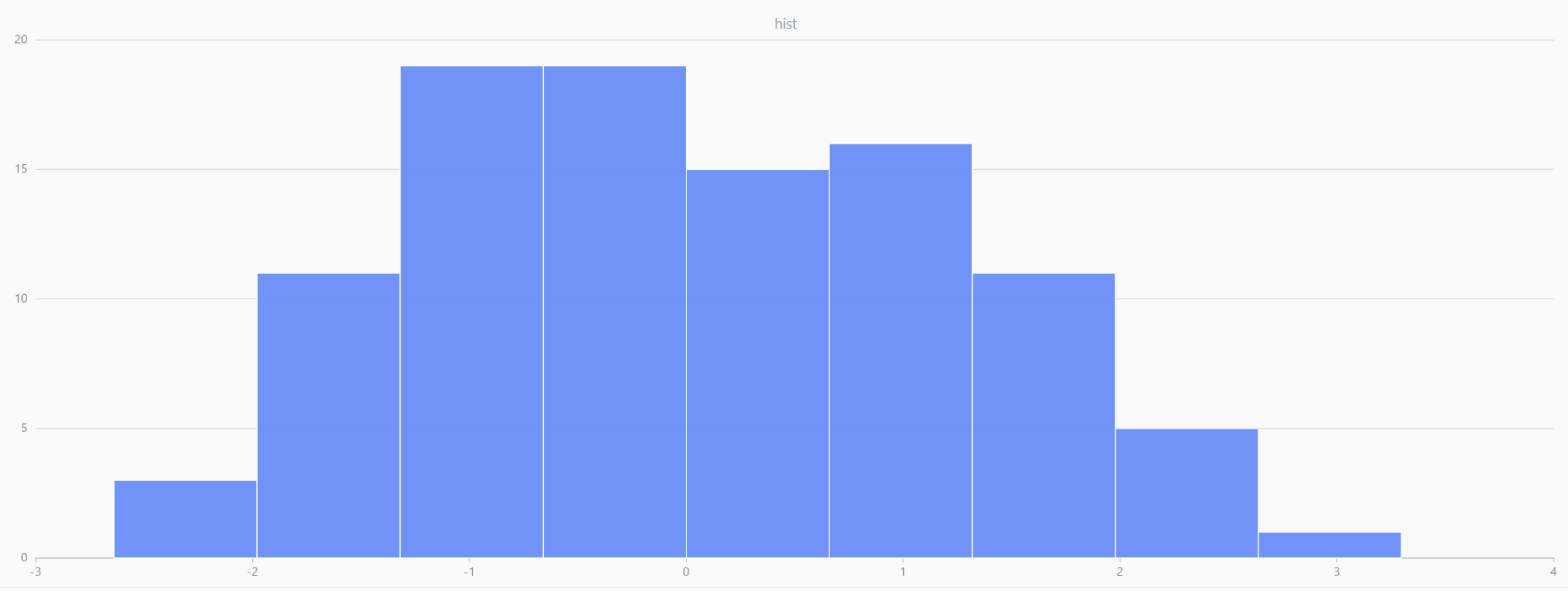
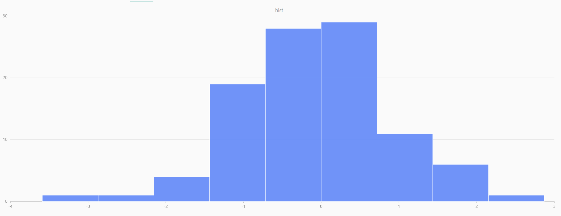
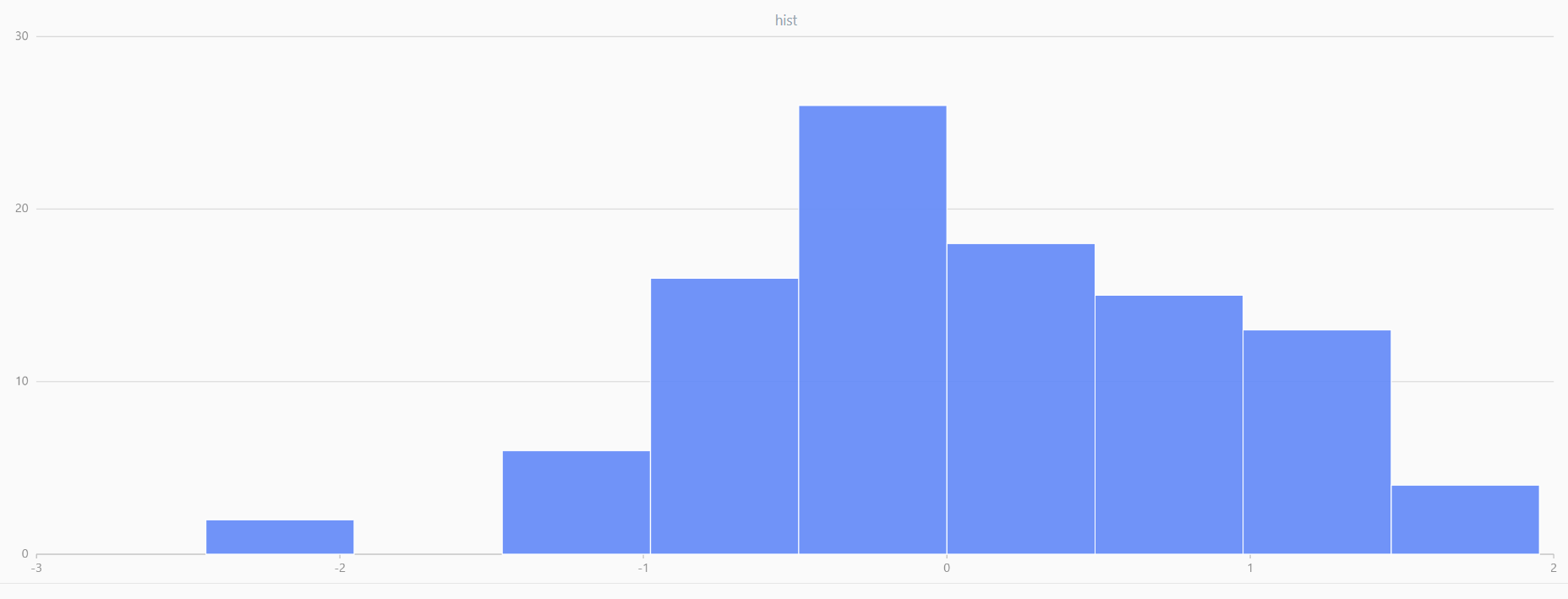
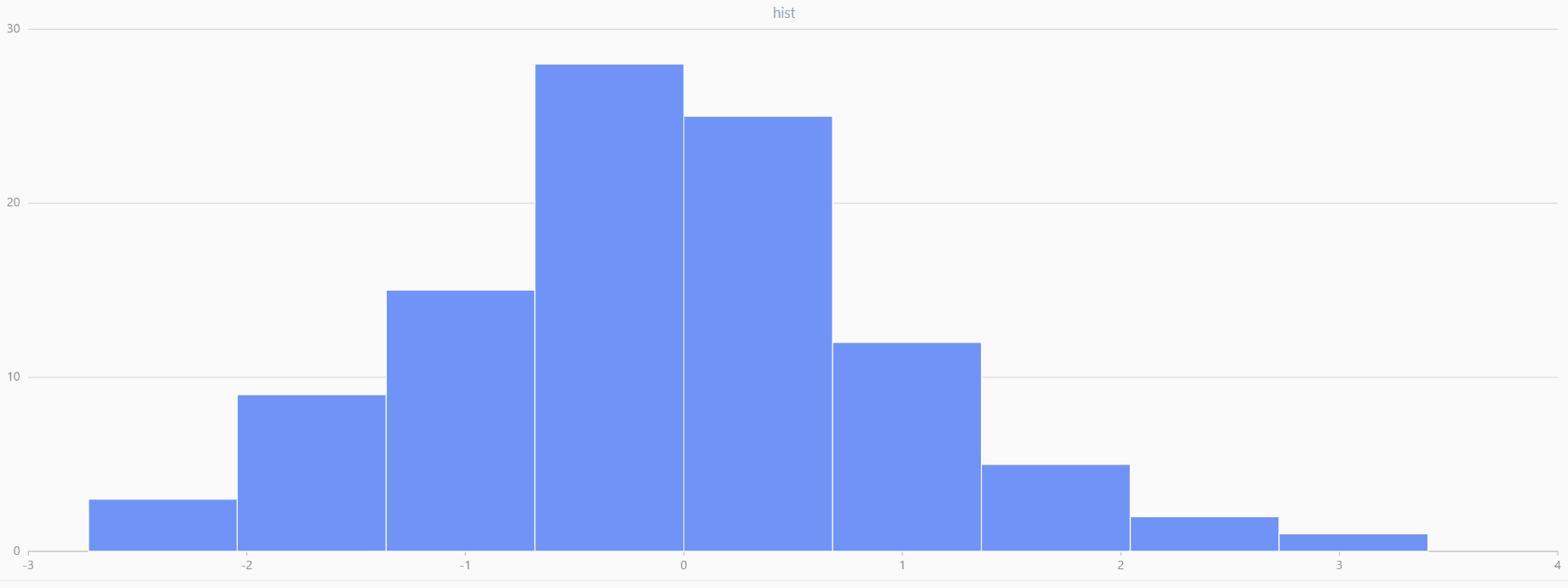
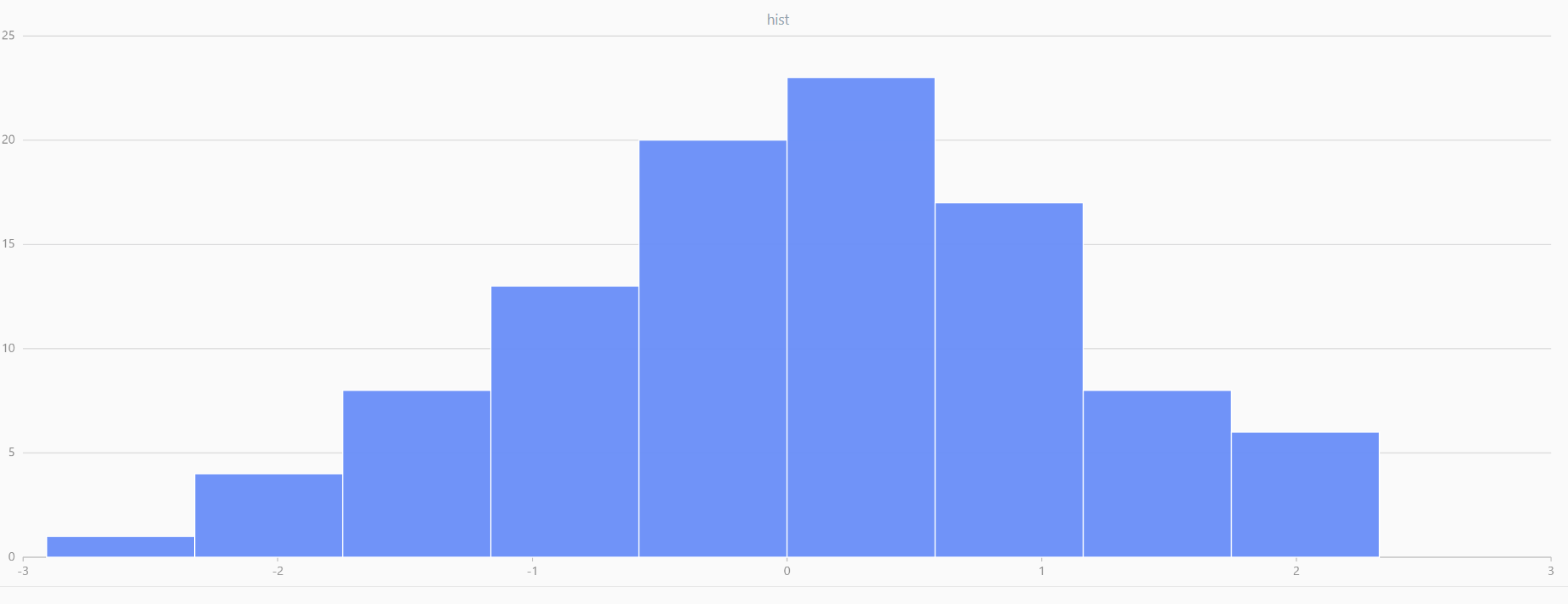
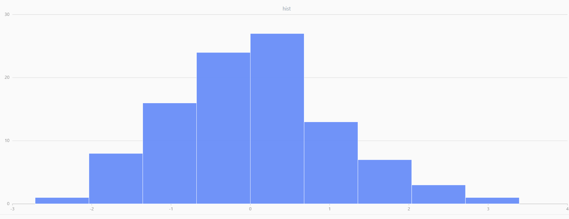
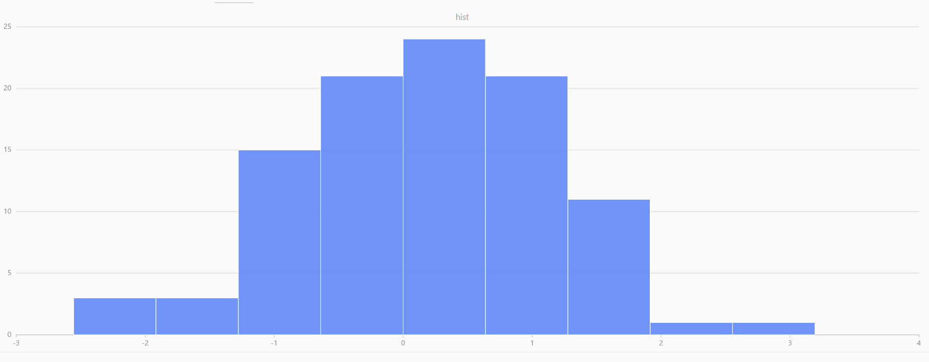
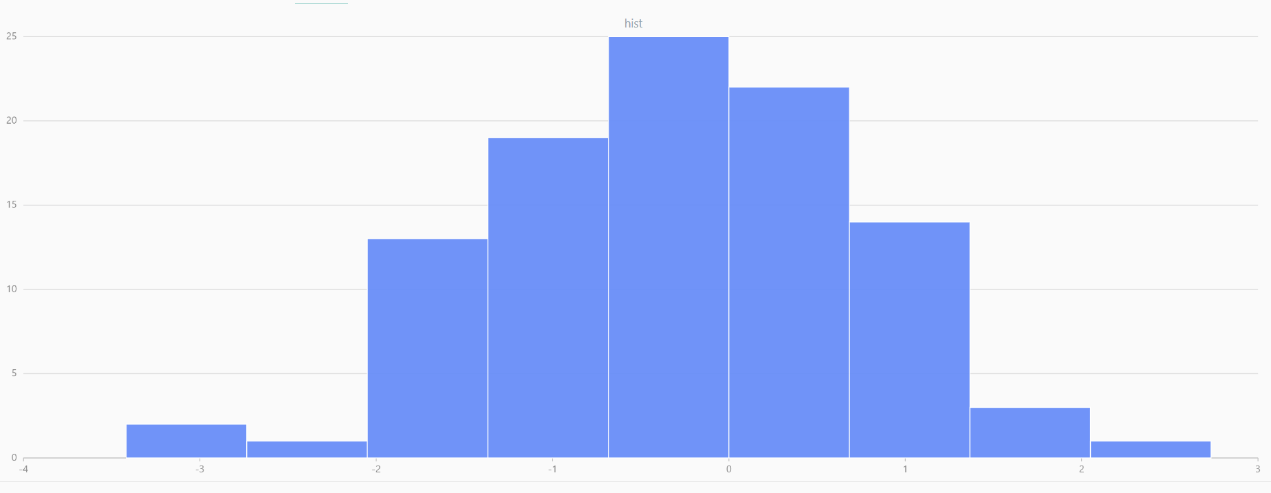
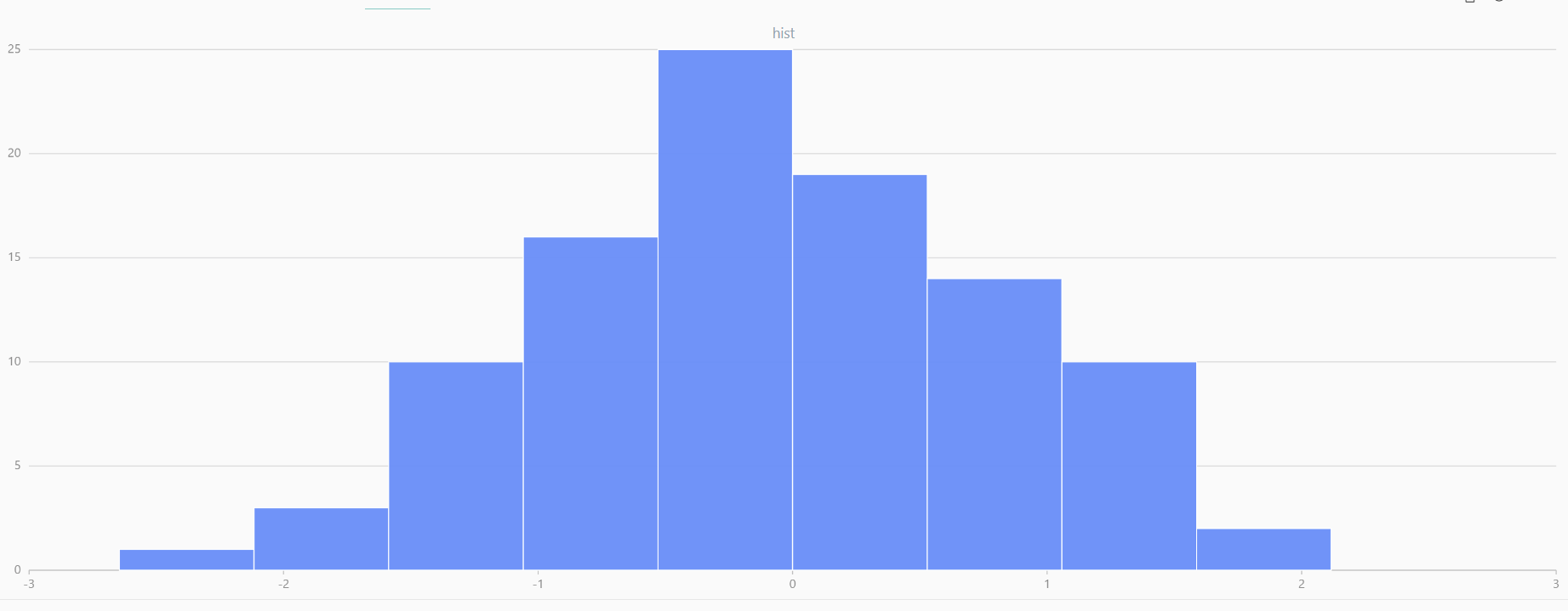
For smaller sample sizes, the variability in the sample distribution is larger. For example, drawing 100 sample points from N(0,1) repeatedly tends to form a normal distribution for the means, but individual samples may deviate significantly.
The randNormal function generates multiple sample groups. Below
is an example generating 20 groups, each containing 100 sample points:
// run 20 times
plot(randNormal(0.0, 1.0, 100), , "hist", HISTOGRAM)
plot(norm(0.0, 1.0, 100), , "hist", HISTOGRAM)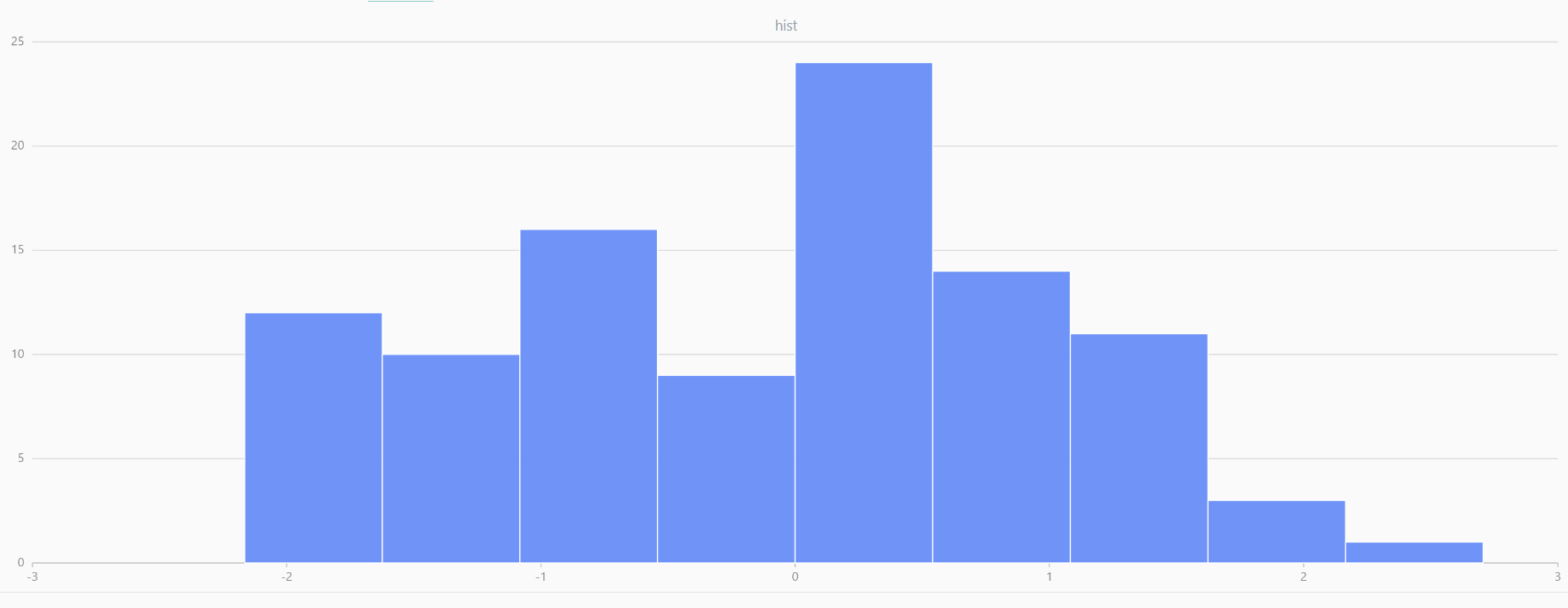 |
 |
 |
 |
 |
 |
 |
 |
 |
 |
 |
 |
 |
 |
 |
 |
 |
 |
 |
 |
| Twenty Distributions of 100 Sample Points Generated from the Standard Normal Distribution | ||||
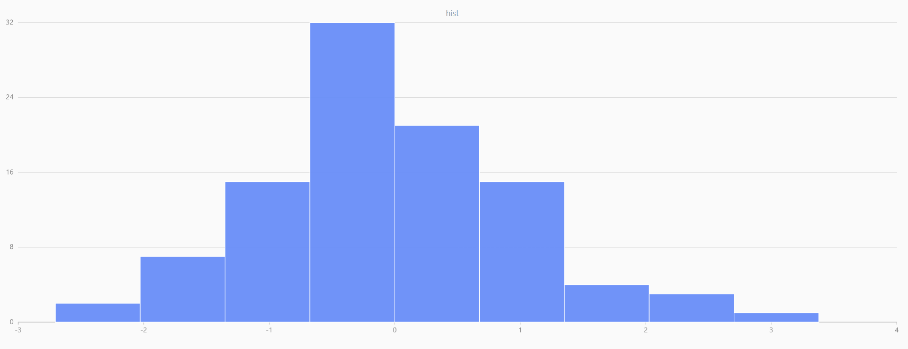
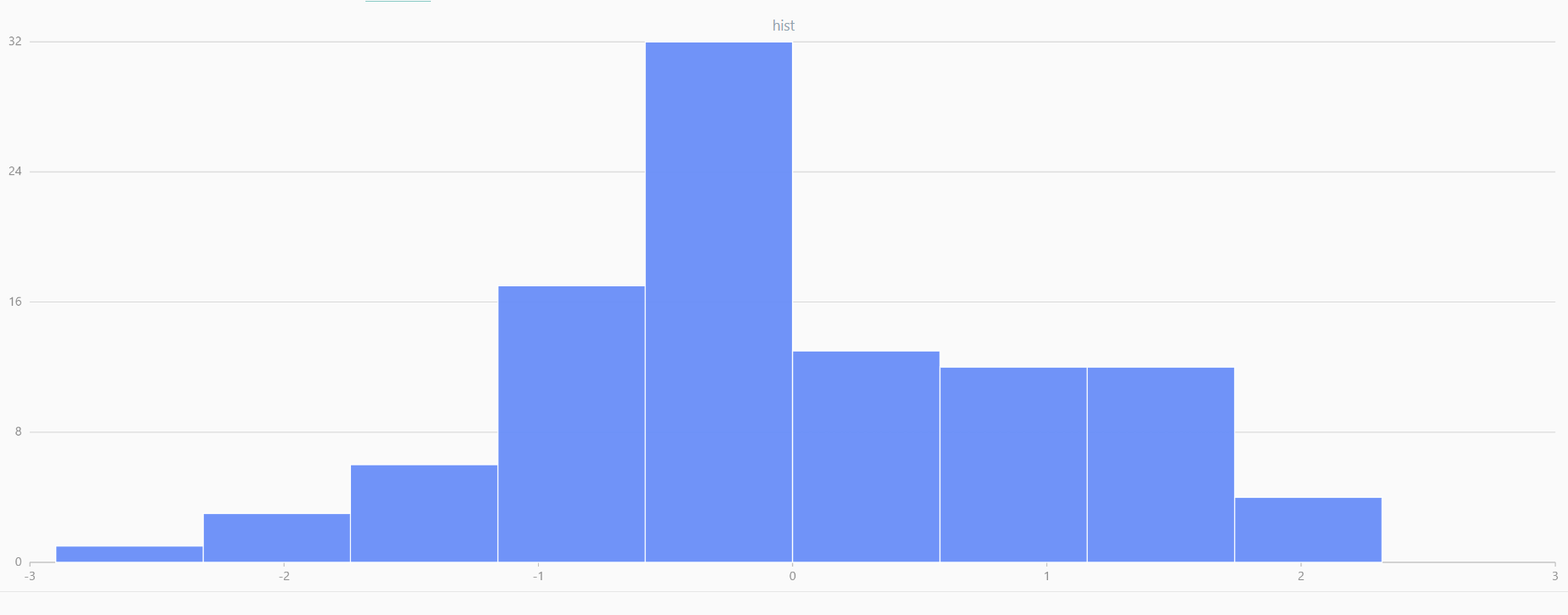
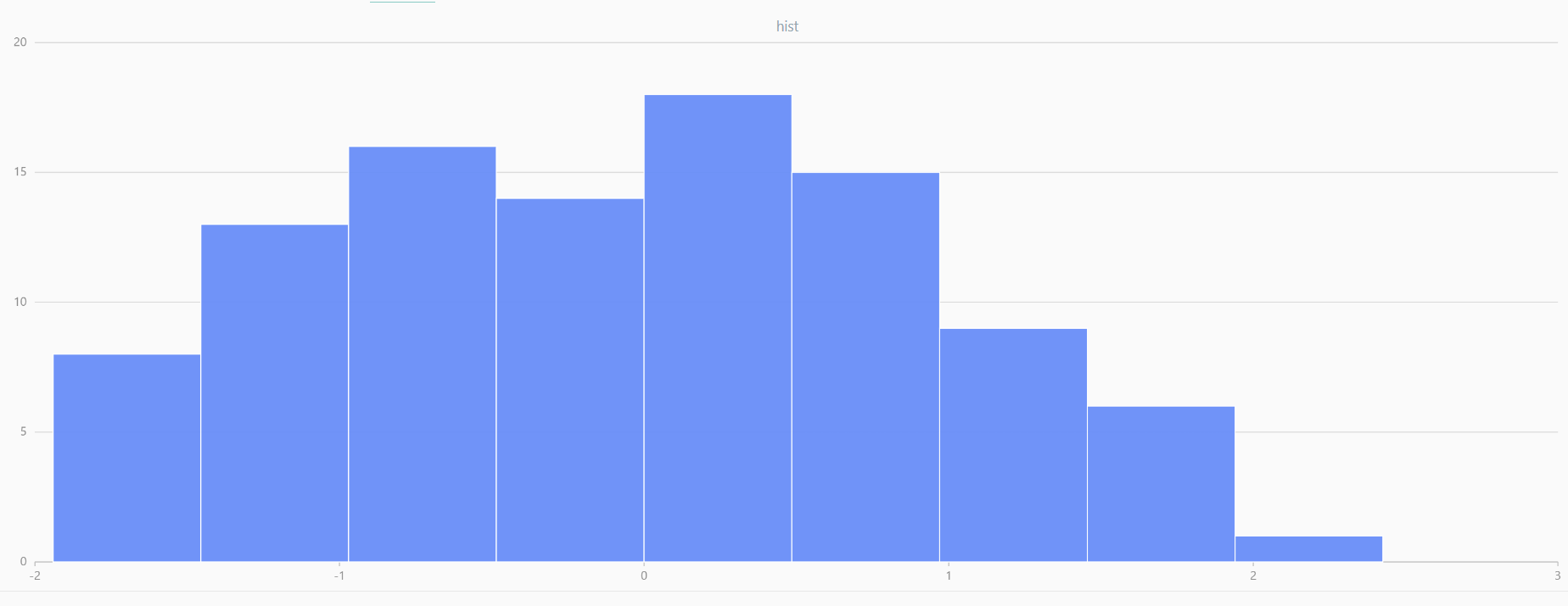
Central Limit Theorem
The Central Limit Theorem (CLT) states that the sum (or difference) of multiple independent random variables X1 , X2 , ... , Xn ∈N (μ, σ) that follow the same normal distribution also follows a normal distribution, i.e.,

Additionally, for independent random variables {Xi} , even if the data does not follow a normal distribution, the sum will assume a near-normal or normal distribution N(nμ, n2σ2) if the sample size is large enough.
In DolphinDB, by applying limit-averaging to multiple uniformly distributed data sets, it can be observed that as the number of distributions increases, the means of these random variables gradually converge to a smooth and nearly normal distribution.
def meanUniform(left, right, n, samples){
setRandomSeed(123)
result = []
for (i in 0 : samples){
result.append!(randUniform(left, right, n))
}
return matrix(result).transpose().mean()
}
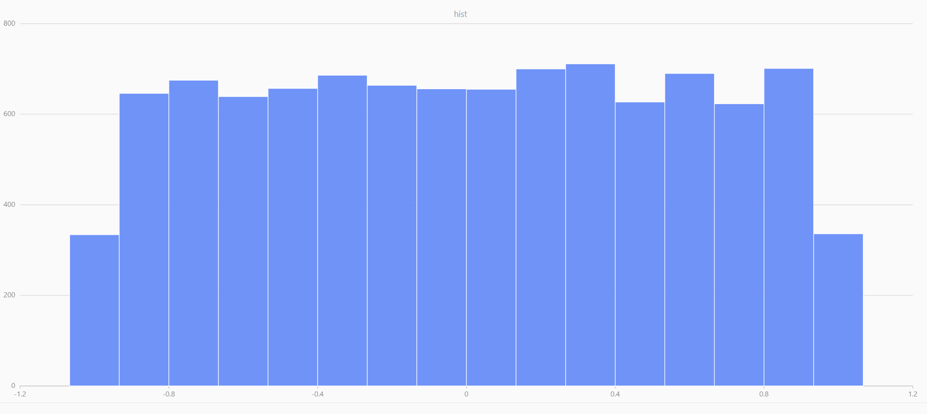
x = randUniform(-1.0, 1.0, 1000000)
plot(x, , "hist", HISTOGRAM)
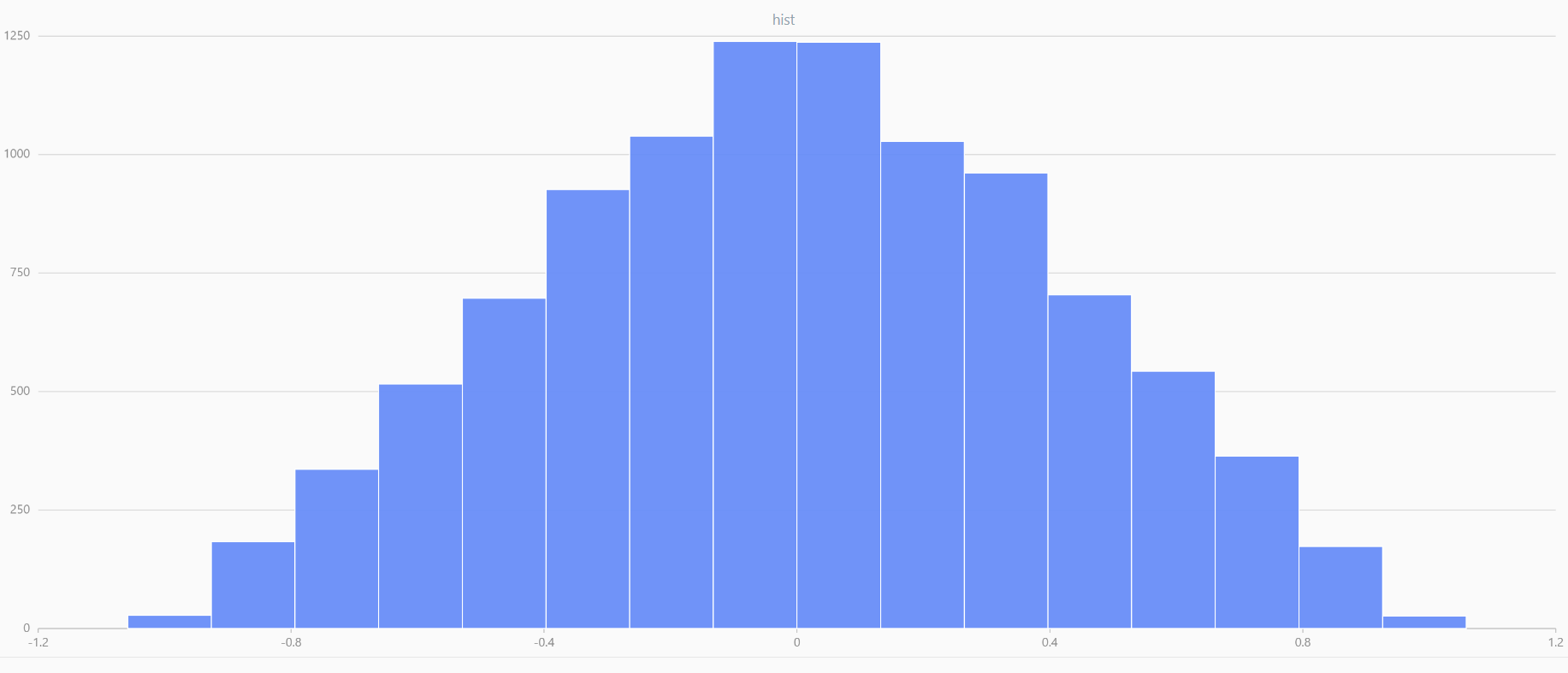
x = meanUniform(-1.0, 1.0, 1000000, 2)
plot(x, , "hist", HISTOGRAM)
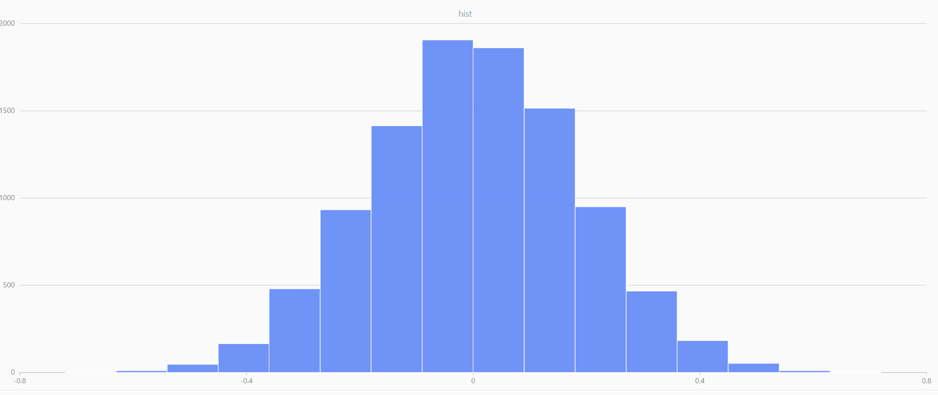
x = meanUniform(-1.0,1.0,1000000, 10)
plot(x, , "hist", HISTOGRAM)
|
|
|
Application: Log-Normal Distribution
The log-normal distribution is widely used in finance to model the behavior of
asset prices and returns. Empirical evidence suggests that long-term log-returns
(e.g., annual or monthly returns) of stocks approximate a normal distribution.
In DolphinDB, log-returns can be simulated using the norm
function.
logreturns = norm(0, 1, 1000).sort()
returns = exp(logreturns).sub(1).sort()
t = select * from table(logreturns, returns) where returns<0.5 and returns>-0.5
plot([t.logreturns, t.returns], t.returns)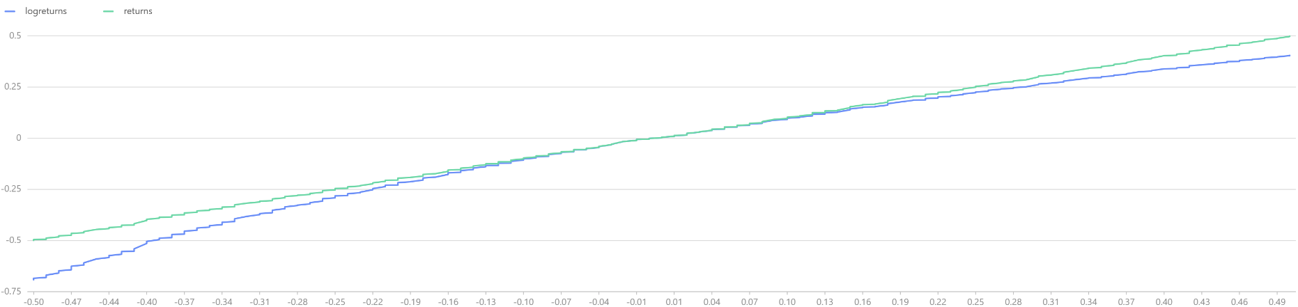
The above comparison between log-returns and regular returns reveals that within the range of -10% to +10%, both distributions largely overlap. However, as the absolute value of the return increases, the regular returns begin to stabilize, while the log-returns continue to maintain their normal distribution characteristics.
Log-returns are additive across time periods. The overall log-return for T
periods is the sum of individual period log-returns. By the central limit
theorem, assuming the logarithmic returns of different periods are independent
and identically distributed, it can be inferred that as T increases,  will gradually converge to the expectation.

When plotting the log-return curve for T periods, it is observed that as T
increases, the log-returns gradually converge, but the converged return  is not fixed. Therefore, if initial capital
X0 is invested for the long term, it is important to focus on the
trend of long-term returns, as greater returns in the final period
is not fixed. Therefore, if initial capital
X0 is invested for the long term, it is important to focus on the
trend of long-term returns, as greater returns in the final period  are desirable. To maximize returns, investors need
to consider two factors: on one hand, the investment horizon T should be
sufficiently long to allow the returns to converge; on the other hand, the Kelly
Criterion can be applied to maximize the expected value of the converging
returns
are desirable. To maximize returns, investors need
to consider two factors: on one hand, the investment horizon T should be
sufficiently long to allow the returns to converge; on the other hand, the Kelly
Criterion can be applied to maximize the expected value of the converging
returns  .
.
dates = getMarketCalendar("CFFEX", 2010.01.01, 2023.12.31)
logreturns = norm(0, 1, dates.size()).sort()
plot(logreturns, dates)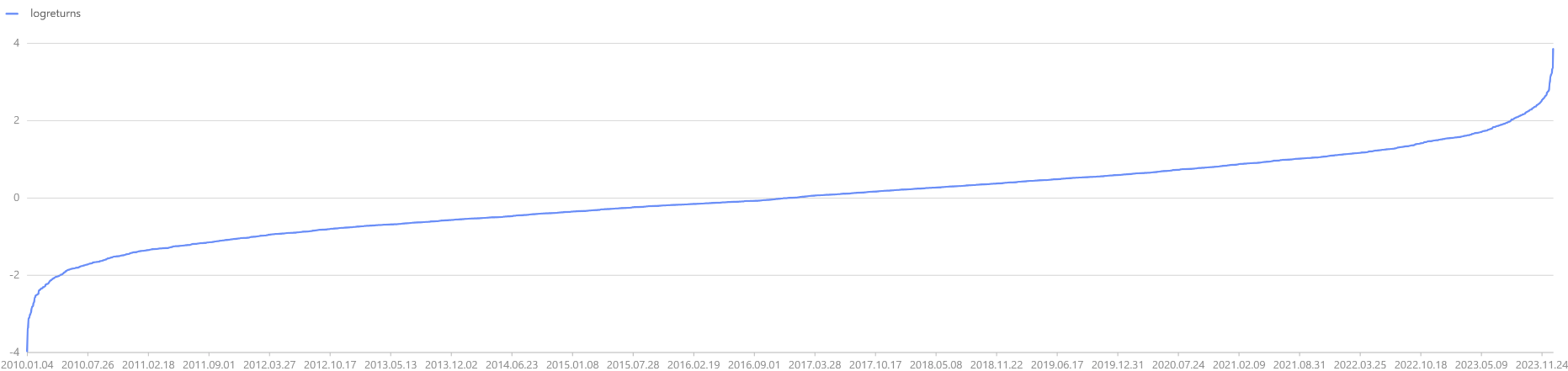
2.3 Continuous Distributions
2.3.1 t-Distribution
The t-distribution is widely used in statistics, particularly when making inferences when the population mean and variance is unknown. If x̄ is the sample mean and s is the sample standard deviation, the resulting t statistic is expressed as:

A common application of the t-distribution is in calculating the confidence
interval for the mean. In DolphinDB, the critical value corresponding to the
t statistic can be obtained using the invStudent function.
For example, assuming a sample size of n=20, the degrees of freedom df=19,
and a significance level of 95%, the critical value corresponding to
tα/2 can be calculated using invStudent(19,
0.975).
x = randNormal(-100, 1000, 10000)
n = x.size()
df = n-1
rt = invStudent(df, 0.975)
// output: 1.9602012636
2.3.2 Chi-Square Distribution
If a random variable X∈N(μ , σ), then  . The sum of squares of n independent standard
normal random variables follows a Chi-Square distribution with n degrees of
freedom:
. The sum of squares of n independent standard
normal random variables follows a Chi-Square distribution with n degrees of
freedom:

When the sample size is small, the ratio of the sample standard deviation S2 to the population standard deviation σ2 also follows a Chi-Square distribution, expressed as:

For example, consider stock returns with a restricted volatility
σ2=0.05. To analyze whether the standard deviation exceeds
the permissible value, the critical value of the Chi-Square statistic can be
calculated using DolphinDB's invChiSquare function. The
analysis shows that the Chi-Square statistic does not exceed the 95%
significance level critical value, so the null hypothesis S2
<=σ2 cannot be rejected. This implies that the sample
return volatility is preliminarily inferred to be within the specified
range.
setRandomSeed(123)
x = randUniform(-0.1, 0.1, 100)
test = (x.size() - 1) * pow(x.std(), 2) \ 0.05
test > invChiSquare(x.size() - 1, 0.95)
// output: false
F-Distribution
The F-distribution is named after Ronald Fisher, who introduced it to determine critical values in ANOVA (Analysis of Variance). By calculating the ratio of variances from two investment portfolios, the F-distribution helps assess whether the two portfolios exhibit the same risk level:

In this context, Sx2 and Sy2 represent the sample standard deviations of the stock returns from the two portfolios, and the distribution of their ratio is the F-distribution. In ANOVA applications, the critical value of the F-distribution is determined based on the degrees of freedom of the numerator and denominator and the significance level, as shown below:

In DolphinDB, the critical value of the F-distribution can be calculated
using the invF function. Assuming that the two investment
portfolios come from different Gaussian distributions, with the latter
having a higher standard deviation, the compareTwoSamples
function is used to perform an F-test. The result indicates that we can
reject the null hypothesis σ1 = σ2, which matches the
expected outcome.
setRandomSeed(1)
x1 = randNormal(0, 1, 20)
x2 = randNormal(0, 5, 30)

def compareTwoSamples(x1, x2, alpha){
   test = (pow(x1.std(), 2)\(x1.size()-1))\(pow(x2.std(), 2)\(x2.size()-1))
   return test > invF(x1.size()-1, x2.size()-1, 1-alpha\2) ||
          test < invF(x1.size()-1, x2.size()-1, alpha\2)
}

compareTwoSamples(x1, x2, 0.05)
// output: true
3. Random Number Generation
DolphinDB not only supports random number generation using the rand
function but also allows generating random numbers from specific probability
distributions. Below is a list of commonly used random number generator functions in
DolphinDB. This section provides detailed instructions on generating random numbers
from specific distributions, performing random sampling, and simulating the price
movement of Snowball options in DolphinDB.
| Function | Usage | Return Value |
|---|---|---|
rand |
rand(X, count) |
Returns a vector of elements randomly selected from X. |
randDiscrete |
randDiscrete(v, p, count) |
Generates random samples from vector v based on the given probability distribution p. |
randUniform |
randUniform(lower, upper,
count) |
Generates the specified number of uniformly distributed random numbers. |
randNormal |
randNormal(mean, stdev,
count) |
Generates the specified number of normally distributed random numbers. |
randBeta |
randBeta(alpha, beta,
count) |
Generates the specified number of random numbers following a Beta distribution. |
randBinomial |
randBinomial(trials, p,
count) |
Generates the specified number of random numbers following a Binomial distribution. |
randChiSquare |
randChiSquare(df, count) |
Generates the specified number of random numbers following a Chi-square distribution. |
randExp |
randExp(mean, count) |
Generates the specified number of random numbers following an Exponential distribution. |
randF |
randF(numeratorDF, denominatorDF,
count) |
Generates the specified number of random numbers following an F-distribution. |
randGamma |
randGamma(shape, scale,
count) |
Generates the specified number of random numbers following a Gamma distribution. |
randLogistic |
randLogistic(mean, s,
count) |
Generates the specified number of random numbers following a Logistic distribution. |
randMultivariateNormal |
randMultivariateNormal(mean, covar, count,
[sampleAsRow=true]) |
Generates random numbers following a multivariate normal distribution. |
randPoisson |
randPoisson(mean, count) |
Generates the specified number of random numbers following a Poisson distribution. |
randStudent |
randStudent(df, count) |
Generates the specified number of random numbers following a t-distribution. |
randWeibull |
randWeibull(alpha, beta,
count) |
Generates the specified number of random numbers following a Weibull distribution. |
3.1 Random Numbers Generation
Generating Random Vectors/Matrices
In DolphinDB, random number vectors can be generated using the
rand function. If X is specified as a scalar, the
generated random numbers will be less than or equal to X and follow a
uniform distribution.
rand(1.0, 10)To generate a random matrix, specify count as a pair of numbers representing the dimensions. For example, the following script generates a 2x2 random matrix:
rand(1.0, 2:2)Generating Random Numbers from Specific Distributions
DolphinDB supports generating random numbers following specific distributions by
providing a suite of generators with the distribution name. For example, to
generate random numbers that follow a normal distribution, you can use the
randNormal function.
fmean, fstd = 0, 1
random_normal_vector = randNormal(fmean, fstd, 10)
random_normal_vector
3.2 Random Sampling
Sampling with Replacement
The rand function supports random sampling with replacement from
the vector X. For example, drawing 5 samples from X:
setRandomSeed(123)
x = 1..10
sample1 = rand(x, 5)
sample1
// output: [7, 8, 3, 5, 3]
Sampling Without Replacement
The shuffle function allows random shuffling of vector X.
By using shuffle, we can implement sampling without
replacement. The following example uses a user-defined function to sample
without replacement from X:
def sampleWithoutReplacement(x,n){
    return x.shuffle()[:n]
}
x = 1..10
sample2 = sampleWithoutReplacement(x, 5)
sample2
Probability Sampling
DolphinDB supports probability sampling by specifying the sampling probabilities
p for each element in the population using the
randDiscrete function. This allows generating random
samples according to a specified probability distribution.
X = `A`B`C`E`F
p = [0.2, 0.3, 0.5, 0.2, 0.2]
randDiscrete(X, p, 5)
3.3 Monte Carlo Simulation: Asset Price Movements
The Monte Carlo simulation for asset price movements assumes that asset prices follow a log-normal distribution. Incorporating the differential equation from the Black-Scholes-Merton (BSM) model, the pricing formula for the asset linked to a Snowball product can be derived as:

Where Δt is the time increment, ST and St represent the asset price at periods T and t, r is the risk-free interest rate, σ is the volatility, and ε is a random variable following a standard normal distribution.
In DolphinDB, Tdays*N random numbers following a standard normal
distribution can be simulated with norm(0, 1, Tdays * N). Using
cumsum for accumulation, the price movements of 128 stocks
can be plotted as shown below.
// Simulation times
N = 1000000
// Underlying asset parameters
vol = 0.13
S0  = 1
r   = 0.03
q   = 0.08
// Date parameters
days_in_year = 240 // Trading days in a year
dt    = 1\days_in_year
all_t = dt + dt * (0..(T * days_in_year - 1))
Tdays = int(T * days_in_year)
// Assume initial asset price is 1
St = 1
S = St * exp( (r - q - vol*vol/2) * repmat(matrix(all_t),1,N) +
    vol * sqrt(dt) * cumsum(norm(0, 1, Tdays*N)$Tdays:N))
// Plot simulated asset price movements
plot(S[,:128].rename!(1..128), 1..(T * days_in_year), "Simulated Stock Price Movements")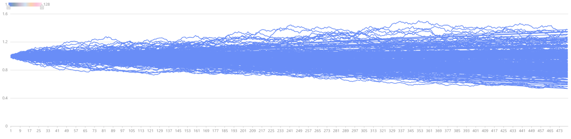
4. Regression
DolphinDB provides a wide range of regression functions to address various regression
scenarios, ranging from simple methods like ols and
wls to advanced techniques. Below is an overview of the
regression functions and their corresponding use cases.
| Function | Regression | Use Case |
|---|---|---|
ols |
Ordinary Least Squares | For standard linear regression problems. |
olsEx |
Ordinary Least Squares | Extends ols to support distributed
computation on partitioned tables. |
wls |
Weighted Least Squares | For handling heteroscedasticity (non-constant error variance) in regression problems. |
logisticRegression |
Logistic Regression | For binary classification problems, predicting probabilities, and classification boundaries. |
randomForestRegressor |
Random Forest Regression | For high-dimensional data and complex relationships in regression problems. |
adaBoostRegressor |
Ensemble Learning Regression | For linear/non-linear relationships and handling outliers in regression tasks. |
lasso |
Lasso Regression | For datasets with many features and for performing feature selection to simplify models. |
ridge |
Ridge Regression | For dealing with multicollinearity among independent variables. |
elasticNet |
Elastic Net Regression | Combines Lasso and Ridge regression, effective for correlated predictors and noise reduction. |
glm |
Generalized Linear Model | Used when the dependent variable is discrete or follows a non-normal distribution. |
5. Hypothesis Testing
In DolphinDB, the steps of hypothesis testing are as outlined below:
- State the null and alternative hypotheses.
- Identify an appropriate test statistic and its distribution and select the corresponding DolphinDB hypothesis testing function.
- Set the confidence level α.
- Use inverse CDF to calculate critical values based on α and the distribution.
- Collect data and calculate the test statistic using DolphinDB’s hypothesis testing functions.
- Compare the test statistic with the critical values to determine whether to reject the null hypothesis and draw a conclusion.
DolphinDB provides a rich set of hypothesis testing functions to address various scenarios.
| Function | Test | Type | Use Case |
|---|---|---|---|
tTest |
t-Test | Parametric Test | Compares whether the means of two samples differ significantly; suitable for normally distributed samples with unknown variance. |
zTest |
z-Test | Parametric Test | Compares whether the means of two samples differ significantly; suitable for normally distributed samples with known variance or large samples. |
fTest |
F-Test | Variance Analysis | Compares whether the variances of two or more samples differ significantly; suitable for normally distributed samples. |
chiSquareTest |
Chi-Square Test | Goodness-of-Fit or Independence Test | Examines differences between observed and expected frequencies; used for both goodness-of-fit and independence tests. |
mannWhitneyUTest |
Mann-Whitney U Test | Non-Parametric Test | Compares the medians of two independent samples; suitable for samples that do not satisfy the normality assumption. |
shapiroTest |
Shapiro-Wilk Test | Normality Test | Tests whether a sample follows a normal distribution; suitable for small sample sizes. |
ksTest |
Kolmogorov-Smirnov Test | Normality or Distribution Fit Test | Tests whether a sample follows a specified distribution or whether two samples come from the same distribution; suitable for large samples. |
5.1 Hypothesis Testing for Mean
5.1.1 z-Test
Using the data from Chapter 4 as an example, the time series graph of stock returns is plotted below.
setRandomSeed(123)
facTable = getAllFactorTable(2, 240)
tmp = select return_day from facTable pivot by record_date, stock_code
plot(tmp[,1:], tmp["record_date"])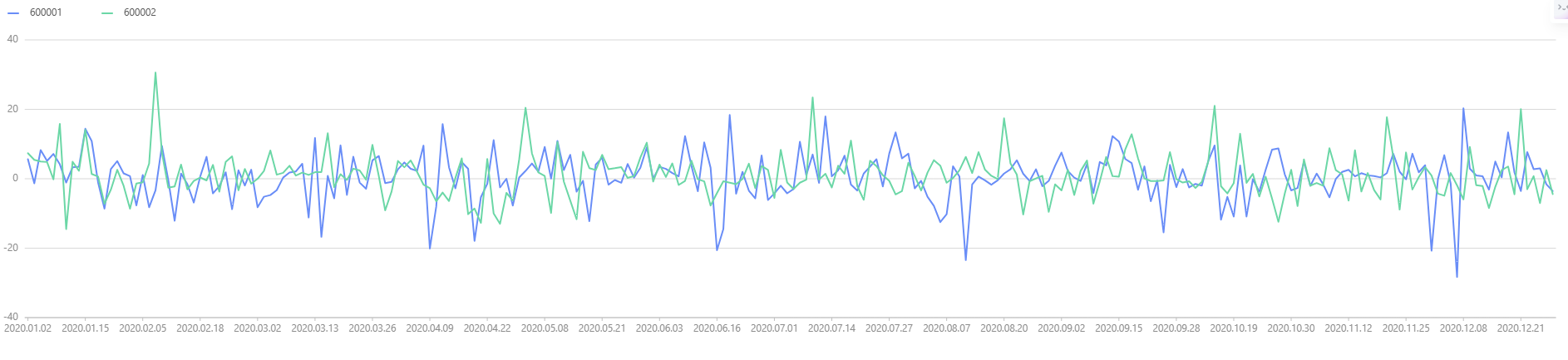
We observe that the returns for both stocks are nearly identical, suggesting that their mean returns may be the same. Next, we perform a hypothesis test to verify this assumption:

Hypothesis: The return samples for both stocks follow a normal distribution, with known variances, and both stocks have a standard deviation of 6.
We use the zTest function to perform the z-test, and the
output is as follows. The calculated z-statistic's p-value is 0.68 (> 0.05),
meaning we fail to reject the null hypothesis, and conclude that the mean
returns of the two stocks are indeed the same.
zTest(tmp["600001"], tmp["600002"], 0, 6, 6)
/* output:
method: 'Two sample z-test'
zValue: 0.4050744166
confLevel: 0.9500000000
stat:
alternativeHypothesis	pValue	lowerBound	upperBound
0	difference of mean is not equal to 0	0.6854233525	-0.8516480908	1.2953848817
1	difference of mean is less than 0	0.6572883237	-∞	1.1227918307
2	difference of mean is greater than 0	0.3427116763	-0.6790550398	∞
*/
5.1.2 t-Test
In practice, since the volatility of stock returns is unknown and the sample
size is typically small, the t-test should be used instead of z-test. Using
DolphinDB's tTest function, the output is as follows. The
calculated t-statistic's p-value is 0.13 (> 0.05), so we fail to reject the
null hypothesis, concluding that the mean returns of the two stocks are
indeed the same.
tTest(tmp["600001"], tmp["600002"], 0)
/* output:
method: 'Welch two sample t-test'
tValue: -0.6868291027
df: 473.7980010389
confLevel: 0.9500000000
stat:
    alternativeHypothesis	pValue	lowerBound	upperBound
0	difference of mean is not equal to 0	0.1314	-2.0292	0.2651
1	difference of mean is less than 0	0.0657	-∞	0.0801
2	difference of mean is greater than 0	0.9342	-1.8441	∞
*/
5.2 Hypothesis Testing for Variance
Variance and standard deviation are essential metrics in finance for assessing risk. Hypothesis tests for variance utilize the chi-square and F-tests.
5.2.1 Chi-Square Test
Using the dataset mentioned above, test if the volatility (variance) of stock 600001's returns is greater than a specific threshold (6). The null and alternative hypotheses are:

The chi-square statistic is calculated using the following formula, and the
critical value at the 95% significance level is obtained using DolphinDB's
invChiSquare function. The results show that the
chi-square statistic is less than the critical value, so we fail to reject
the null hypothesis, concluding that the volatility of stock 600001 is not
greater than 6.

test_statistic =(size(tmp)-1)*tmp["600001"].var()/36
print(stringFormat("chi-squre test statistic:%.2F",test_statistic))
chi_statistic=invChiSquare(size(tmp)-1,0.95)
print(stringFormat("chi-squre test statistic:%.2F",chi_statistic))
/* output:
chi-squre test statistic:233.59
chi-squre test statistic:276.06
*/
5.2.2 F-Test
To compare whether the volatilities (variances) of returns for two stocks are consistent, an F-test can be used. The null and alternative hypotheses are as follows:

Using DolphinDB's fTest function, the F-test output is as
follows. Based on the analysis, the calculated F-statistic is 0.79, which
lies between the left and right critical values of the F-distribution.
Therefore, we fail to reject the null hypothesis, concluding that the
variances of the returns for the two stocks are equal.
fTest(tmp["600001"], tmp["600002"])
/*Output
method: 'F test to compare two variances'
fValue: 0.7907099827
numeratorDf: 239
denominatorDf: 239
confLevel: 0.9500000000
stat:
	alternativeHypothesis	pValue	lowerBound	upperBound
0	ratio of variances is not equal to 1	0.0701139943	0.6132461206	1.0195291184
1	ratio of variances is less than 1	0.0350569972	0.0000000000	0.9786251182
2	ratio of variances is greater than 1	0.9649430028	0.6388782232	∞
*/