Latency Measurement and Performance Improvement of Stream Computing
In real-time computing, end-to-end response latency is the most critical metric for evaluating computing performance. DolphinDB’s built-in streaming data framework supports data publishing and subscribing, incremental stream computation, real-time joins, and more. This allows users to efficiently implement complex real-time computing jobs with millisecond-level or even sub-millisecond-level latency without writing large amounts of code.
This tutorial introduces how to measure end-to-end latency for DolphinDB streaming jobs and how to optimize scripts for low-latency real-time computation.
1. Latency Measurement
By recording timestamps at key stages in the processing pipeline, we can measure the latency at each step of stream computing. In addition, DolphinDB’s streaming engines provide a built-in latency measurement feature, offering more details to support further analysis and performance optimization.
1.1 Use the now Function to Record Processing Timestamps
At key points such as data publishing, receiving, and outputting results, users
can use the now function to get the current timestamp and store
it in the table. The script below demonstrates this approach:
// create engine and subscribe
share streamTable(1:0, `sym`time`qty`SendTime, [STRING, TIME, DOUBLE, NANOTIMESTAMP]) as tickStream
result = table(1000:0, `sym`time`factor1`SendTime`ReceiveTime`HandleTime, [STRING, TIME, DOUBLE, NANOTIMESTAMP, NANOTIMESTAMP, NANOTIMESTAMP])
dummyTable = table(1:0, tickStream.schema().colDefs.name join `ReceiveTime, tickStream.schema().colDefs.typeString join `NANOTIMESTAMP)
rse = createReactiveStateEngine(name="reactiveDemo", metrics =[<time>, <cumsum(qty)>, <SendTime>, <ReceiveTime>, <now(true)>], dummyTable=dummyTable, outputTable=result, keyColumn="sym")
def addHandleTime(mutable msg){
update msg set ReceiveTime = now(true)
getStreamEngine("reactiveDemo").append!(msg)
}
subscribeTable(tableName="tickStream", actionName="addTimestampDemo", offset=-1, handler=addHandleTime, msgAsTable=true)
// generate input data
data1 = table(take("000001.SZ", 5) as sym, 09:30:00.000 + [0, 1, 5, 6, 7] * 100 as time, take(10, 5) as qty)
data2 = table(take("000002.SZ", 3) as sym, 09:30:00.000 + [2, 3, 8] * 100 as time, take(100, 3) as qty)
data3 = table(take("000003.SZ", 2) as sym, 09:30:00.000 + [4, 9] * 100 as time, take(1000, 2) as qty)
data = data1.unionAll(data2).unionAll(data3).sortBy!(`time)
// insert data into engine
update data set SendTime = now(true)
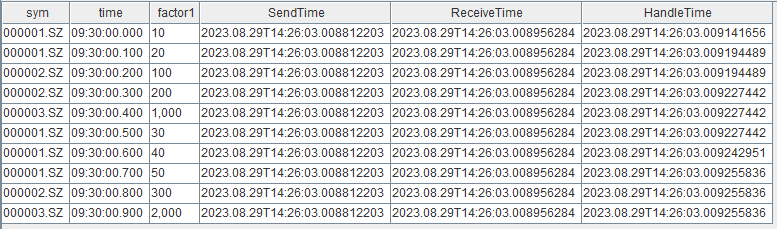
tickStream.append!(data)In the result table, SendTime records the time when data is
injected into the publishing stream table, ReceiveTime records
the time when subscriber receives the data, and HandleTime
records the time when reactive state engine completes factor computation.
When using now function in the metrics parameter of
streaming engines, keep the following in mind:
- Specify
now()as the last element of metrics. It captures the time when the computation of the output record is completed before writing it into the output table (the write latency is not included). - For time-series aggregation engines
(
createTimeSeriesEngine/createDailyTimeSeriesEngine/createSessionWindowEngine), note the following:- You can use the
nowfunction directly in the metrics parameter of aggregation engines. Make sure not to wrapnow()inside an aggregation function. - In versions prior to 2.00.10 / 1.30.23, if multiple groups trigger
output at the same time (e.g., when useSystemTime = true), the
engine would call
now()once for each group. In later versions, the optimized aggregation engine callsnow()only once for the entire batch of grouped outputs.
- You can use the
1.2 Use timer Statement to Verify Streaming Engine
Performance
Inject a batch of data into the engine and use the timer
statement to measure total processing time from data injection to completion of
calculation. This approach is useful for quickly validating engine performance
during factor development and optimization. For specific implementation, refer
to Stream Processing of
Financial Factors, which compares the performance of 4 different
implementations of the same factor using the timer
statement.
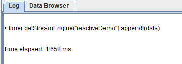
timer getStreamEngine("reactiveDemo").append!(data)- The
timerstatement measures execution time of a single command. - When appending data to the engine, the operation is synchronous: once the append statement completes, the engine has finished processing the batch.
- It is recommended to inject batch data to evaluate total processing latency.
- When injecting only a few records (e.g. one record), the characteristics of
input data and differences between different engines must be considered.
- Reactive state engines produce output on a per-record basis, so injecting any single record will trigger and output corresponding results, reflecting the single-response latency of the reactive state engine.
- However, for time-series aggregation engines using non-system event triggers (useSystemTime=false), not every batch of data will generate output. To measure the single-response latency in such cases, specific data with timestamps that can trigger output must be injected.
Example script:
// create engine
def sumDiff(x, y) {
	return (x-y)/(x+y)
}
factor1 = <ema(1000 * sumDiff(ema(price, 20), ema(price, 40)),10) -  ema(1000 * sumDiff(ema(price, 20), ema(price, 40)), 20)>
share streamTable(1:0, `sym`time`price, [STRING, TIME, DOUBLE]) as tickStream
result = table(1000:0, `sym`time`factor1, [STRING, TIME, DOUBLE])
rse = createReactiveStateEngine(name="reactiveDemo", metrics =[<time>, factor1], dummyTable=tickStream, outputTable=result, keyColumn="sym")
// generate input data
data1 = table(take("000001.SZ", 100) as sym, 09:30:00 + 1..100 *3 as time, 10+cumsum(rand(0.1, 100)-0.05) as price)
data2 = table(take("000002.SZ", 100) as sym, 09:30:00 + 1..100 *3 as time, 20+cumsum(rand(0.2, 100)-0.1) as price)
data3 = table(take("000003.SZ", 100) as sym, 09:30:00 + 1..100 *3 as time, 30+cumsum(rand(0.3, 100)-0.15) as price)
data.append!(data1.unionAll(data2).unionAll(data3).sortBy!(`time))
// test perfomance
timer getStreamEngine("reactiveDemo").append!(data)
Timing statistics in GUI:
1.3 Use outputElapsedMicroseconds Parameter to Calculate Detailed Timing of Streaming Engines
Starting from versions 2.00.9 / 1.30.21, several streaming engines support the
outputElapsedMicroseconds parameter, which provides detailed internal
timing statistics. Supported engines include
createTimeSeriesEngine,
createDailyTimeSeriesEngine,
createReactiveStateEngine, and
createWindowJoinEngine.
Example:
// create engine
share streamTable(1:0, `sym`time`qty, [STRING, TIME, LONG]) as tickStream
result = table(1000:0, `sym`cost`batchSize`time`factor1`outputTime, [STRING, LONG, INT, TIME, LONG, NANOTIMESTAMP])
rse = createReactiveStateEngine(name="reactiveDemo", metrics =[<time>, <cumsum(qty)>, <now(true)>], dummyTable=tickStream, outputTable=result, keyColumn="sym", outputElapsedMicroseconds=true)
// generate input data
data1 = table(take("000001.SZ", 5) as sym, 09:30:00.000 + [0, 1, 5, 6, 7] * 100 as time, take(10, 5) as qty)
data2 = table(take("000002.SZ", 3) as sym, 09:30:00.000 + [2, 3, 8] * 100 as time, take(100, 3) as qty)
data3 = table(take("000003.SZ", 2) as sym, 09:30:00.000 + [4, 9] * 100 as time, take(1000, 2) as qty)
data = data1.unionAll(data2).unionAll(data3).sortBy!(`time)
// insert data into engine
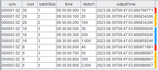
getStreamEngine("reactiveDemo").append!(data)The result table shows cost and batchSize
columns as timing details. The cost column represents the
processing time (in microseconds) for each batch, and batchSize
shows how many records were processed in that batch.
In this example, 10 input records were processed as 5 batches. This batching behavior is determined by the input data and how the reactive state engine groups data for processing. Within the same group, the reactive state engine processes input data on a per-record basis, while different groups are processed in the same batch for vectorized processing. Therefore, we can see that the first record with grouping column 000001.SZ is processed as a separate batch, followed by the second 000001.SZ record and subsequent 000002.SZ records calculated and output in the same batch.
To calculate total processing time for the injected 10 records:
select sum(cost\batchSize) as totalCost from result2. Performance Optimization
In DolphinDB's streaming framework, real-time data is first injected into streaming tables, then based on the publish-subscribe-consume model, the publisher actively pushes incremental input data to consumers, continuously executing specified processing functions for computation through callbacks on message processing threads, and writing calculation results to tables. Throughout the entire computation pipeline, we find optimization opportunities in three aspects: writing, computation, and framework design.
2.1 Writing
Streaming tables are a core component of DolphinDB’s streaming framework. Throughout the computation chain, there are multiple writes to streaming tables: for example, records continuously generated from external devices or trading systems are written to streaming tables in real-time as input for subsequent real-time computation; additionally, computed results from streaming engines are also written into tables. Since write latency contributes to total processing latency, optimizing write performance can help reduce end-to-end latency.
Pre-allocate Memory When Creating Tables
- Regular shared streaming tables
Specify a sufficiently large capacity parameter when creating the table. For example, for stock market data, you can estimate the daily data volume based on historical data and set the capacity slightly larger than this value.
capacity = 1000000
share(streamTable(capacity:0, `sym`time`price, [STRING,DATETIME,DOUBLE]), `tickStream)
The capacity parameter of
streamTablespecifies the number of records for which memory is initially allocated. When the record count exceeds capacity, the system reallocates memory at 1.2 times the current capacity, copies existing data to the new space, releases the old space, and continues writing.Since memory allocation and data copying are costly operations, each expansion may cause latency spikes. For instance, if capacity is set too small (e.g., 1), frequent memory expansions will occur as data grows, and each subsequent expansion becomes more time-consuming due to the larger data size being copied.
- Persistent streaming tables
Specify reasonable values for cacheSize and capacity when creating persistent streaming tables. If memory resources are sufficient, set cacheSize and capacity based on estimated daily data volume.
cacheSize = 1000000
enableTableShareAndPersistence(table=streamTable(cacheSize:0, `sym`time`price, [STRING,DATETIME,DOUBLE]), tableName="tickStream", asynWrite=true, compress=true, cacheSize=cacheSize, retentionMinutes=1440, flushMode=0, preCache=10000)
The cacheSize parameter specifies the maximum number of rows kept in memory. When the number of rows exceeds cacheSize and all data has been flushed to disk, the system reallocates memory for the newest 50% of rows and releases the old memory.Similarly, each memory cleanup operation may cause latency spikes due to memory reallocation and data copying. With sufficient memory, it is recommended to set a large enough cacheSize to keep all data in memory and avoid cleanup operations altogether. If memory control is required, configure cacheSize to balance the frequency and severity of spikes, as its size determines the amount of data to copy during cleanup, directly impacting latency.
2.2 Computation
DolphinDB’s streaming engines are specialized modules for real-time streaming computations, supporting various scenarios such as window aggregation, event-driven processing, etc. When creating a streaming engine, the metrics parameter specifies computation logic in meta-code form, representing real-time indicators implemented in DolphinDB scripts. After selecting the appropriate engine type, optimizing the metrics formula becomes key to improving performance. Therefore, the first three subsections of this section introduce optimization methods for streaming indicator implementation, and the last subsection provides recommendations for scenarios where streaming engines are not necessary.
2.2.1 Built-in State Functions and Incremental Computation
Suppose we receive real-time tick-by-tick transaction data and respond to each transaction record individually, accumulating the latest daily total transaction volume. If each calculation uses all transaction data up to the current point, performance would be poor. However, through incremental streaming implementation, performance can be greatly improved. Specifically, the latest cumulative transaction volume can be obtained by adding the transaction volume of the latest record to the previously calculated transaction volume. This incremental calculation requires historical state (previously calculated transaction volume), which we call stateful computation.
DolphinDB provides numerous built-in state functions in reactive state
engines, time-series aggregation engines, and window join engines. Using
built-in state functions in metrics can implement the above
incremental stateful computation, with historical states automatically
maintained by the engine internally. For example, using the
cumsum function in reactive state engines can implement
incremental accumulation.
For state functions supported by each engine, refer to the user manual for
createTimeSeriesEngine,
createReactiveStateEngine, and
createWindowJoinEngine. It's recommended to prioritize
built-in state functions for implementing real-time indicators with
incremental algorithms.
2.2.2 Just-In-Time (JIT) Compilation
Just-in-time compilation is a form of dynamic compilation that can improve program execution efficiency. DolphinDB’s scripting language is interpreted. When a program runs, it first performs syntax analysis to generate a syntax tree, and then executes it recursively. Without vectorization, the interpretation overhead can be relatively high, because DolphinDB is implemented in C++, and a single function call in the script may translate into multiple virtual function calls in C++.
Since streaming computation tasks are continuously triggered, functions are repeatedly invoked. For example, as described in Section 1.3 on reactive state engines, injecting just 10 records will result in 5 function calls for the metrics. The interpretation overhead accumulates and contributes to the overall processing latency. This is especially significant for reactive state engines, where in some scenarios, a large portion of the total latency may come from interpretation. Therefore, it is recommended to reduce interpretation overhead by implementing JIT functions. For practical examples, please refer to Stream Processing of Financial Factors, which demonstrates performance improvements for a moving average buy-sell pressure factor using JIT.
2.2.3 Array Vector
In DolphinDB, an array vector is a special type of vector used to store variable-length two-dimensional arrays. This data structure can significantly simplify certain common queries and calculations. For details, please refer to Best Practices for Array Vectors.
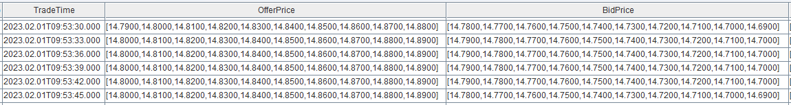
The level-2 order book (10 best bid/ask prices and volumes) is one of the
most important components in market snapshots. When developing
high-frequency factors, vectorized computing on this data is often
desirable. The fixedLengthArrayVector function can be used
to combine 10 best bid/ask data into an array vector. Leveraging this
feature, it is recommended to store these fields directly as array vectors.
This eliminates the need to assemble the 10 best bid/ask data during
function execution, thereby reducing computational latency. For practical
examples, please refer to Stream Processing of
Financial Factors, which demonstrates how array vectors can be
used to optimize the performance of a moving average buy-sell pressure
factor.
2.2.4 Custom Handlers and Stateless Computation
Not all calculations require streaming engines. Simple stateless computations can often be handled directly in custom functions. For example, to process only trades after 09:30, you can filter data in a custom handler before sending it to the engine:
def filterTime(msg){
	tmp = select * from msg where time > 09:30:00.000
	getStreamEngine("reactiveDemo").append!(tmp)
}
subscribeTable(tableName="tickStream", actionName="demo", offset=-1, handler=filterTime, msgAsTable=true)- The same filtering can be achieved by adding another layer of reactive state engine, but due to overhead from grouping and state maintenance within streaming engines, custom functions are more efficient implementations than streaming engines for stateless computation scenarios.
- The handler function processes incremental data each time, meaning the msg variable in the above script is newly added data received by the subscriber, not the latest full snapshot of the tickStream table.
2.3 Framework
In some scenarios, even after optimizing the implementation of individual
indicators to the extreme, large input data volumes may still overwhelm the
system’s processing capacity, resulting in significant response latency. If
input data flow is consistently greater than the system processing capacity,
you'll see continuously increasing queueDepth values
(getStreamingStat().subWorkers) on the subscriber node,
indicating unhealthy streaming tasks that need to be stopped and optimized.
A DolphinDB streaming job consists of stream tables, stream computing engines, and message processing threads. Conceptually, a streaming task can be viewed as a background thread repeatedly executing a computation function. Stream engines or custom functions serve as this computation function, while stream tables trigger background thread invocations via publish-subscribe mechanisms, with each invocation processing the incremental data batch. This section discusses optimization methods from the perspective of streaming task framework design.
2.3.1 Micro-Batch Processing
By setting appropriate batchSize and throttle parameters when
calling subscribeTable, micro-batch processing can be
achieved to improve throughput, reduce blocking, and thus lower latency.
This leverages the fact that per-batch processing time does not increase
linearly with batch size. For example, writing 1000 records to a distributed
database may take almost the same time as writing 10 records. Therefore,
utilizing batch processing can significantly reduce overall latency.
The batchSize and throttle parameters jointly determine consumption triggers, and are evaluated with an OR condition. When the number of unprocessed records in the subscription queue reaches batchSize, consumption is triggered. However, due to possible fluctuations in data arrival rates, there may be times when batchSize is not reached for a while. In such cases, throttle ensures that data accumulated for a specified time is still processed. Both parameters should be adjusted based on data input rates and processing speeds.
Additionally, note the following two points:
- The system configuration subThrottle (in dolphindb.cfg or
cluster.cfg) must be set to 1 to allow throttle values smaller
than 1 second. Otherwise, even if
subscribeTablespecifies throttle as 0.001, the effective value remains 1 second. - It is recommended to always specify both batchSize and
throttle when calling
subscribeTable. If not specified, each batch processed corresponds to the size of data blocks as they arrive in the queue, not the total accumulated data. For example, if 10 unprocessed records arrive in blocks of 2, 3, and 5 records, the worker will process them in three separate batches, rather than one batch of 10 records. Therefore, if records are inserted frequently but in small quantities, failing to configure batchSize and throttle may result in poor performance.
2.3.2 Parallel Processing
The hash parameter of subscribeTable can be
configured to improve parallelism and reduce latency. Each call to
subscribeTable allocates a fixed message processing
thread to its handler function. Proper thread allocation can maximize
CPU utilization. Optimization strategies include:
- Assign different streaming tasks to different processing
threads:
- Whenever possible, assign different tasks to separate threads. If multiple streaming tasks share the same hash value, they are allocated to the same thread and compete for resources, increasing response latency for each task.
- When the number of tasks exceeds available processing threads, prioritize assigning complex (long-running) tasks to separate threads.
- Split a single streaming task into multiple threads:
- For high-volume input streams that cannot be handled by a single thread, data can be partitioned across multiple threads for parallel processing. See Stream for DolphinDB for implementation details. Note that writing results from multiple threads into a shared memory table may involve write locks and waiting. To avoid this, results can be written into separate tables.
dispatchStreamEngineoffers a lightweight alternative tosubscribeTablefor distributing data and parallel processing.
2.3.3 Stream Engine Cascading
In DolphinDB, complex indicators are often decomposed into multiple stages, each handled by a separate engine. Traditionally, intermediate results are stored in intermediate tables, with subsequent engines consuming these results via additional subscriptions. However, this introduces memory and latency overhead. DolphinDB stream engines support the table interface, allowing one engine to directly feed another without intermediate tables—a technique known as stream engine cascading—which offers better performance.
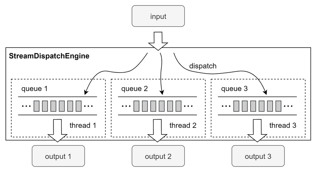
2.3.4 Stream Dispatch Engine
While splitting a task into multiple parallel threads via multiple
subscribeTable subscriptions can improve throughput,
having too many subscriptions may create publishing bottlenecks since there
is only one publisher thread per node. In versions 1.30.22, 2.00.9 and
above, DolphinDB introduced the Stream Dispatch Engine
(createStreamDispatchEngine), which distributes
incoming data across multiple threads and directly injects incremental data
into downstream output tables or engines on those threads.
In the following example, data is subscribed once, then written into a
dispatch engine. The dispatch engine partitions data by the
sym field across three threads for computation using
reactive state engines.
//  create engine
share streamTable(1:0, `sym`price, [STRING,DOUBLE]) as tickStream
share streamTable(1000:0, `sym`factor1, [STRING,DOUBLE]) as resultStream
rseArr = array(ANY, 0)
for(i in 0..2){
	rse = createReactiveStateEngine(name="reactiveDemo"+string(i), metrics =<cumavg(price)>, dummyTable=tickStream, outputTable=resultStream, keyColumn="sym")
	rseArr.append!(rse)
}
dispatchEngine=createStreamDispatchEngine(name="dispatchDemo", dummyTable=tickStream, keyColumn=`sym, outputTable=rseArr, mode="buffer", dispatchType="uniform")
//  subscribe
subscribeTable(tableName="tickStream", actionName="dispatch", handler=dispatchEngine, msgAsTable=true)
How Stream Dispatch Engine Works:
- The outputTable parameter is a list of tables (or engines). When created, an equal number of threads and buffer queues are allocated.
- Each thread processes data from its buffer queue and writes it into the corresponding output table or engine. If dispatching into engines, the calculations are performed directly on these threads.
- These threads are independent of the
subscribeTablemessage processing threads and are not constrained by the subExecutor parameter in system configuration.
Best Practices for Stream Dispatch Engine:
- It is recommended to use the default
mode
"buffer", which processes all unprocessed data in batches — consistent with micro-batch processing best practices. - When using
dispatchType="hash", skewed data distributions may overload some threads. In such cases, usedispatchType="uniform"for even distribution:"hash"works likehashBucketfunction, where each key is consistently mapped to a fixed bucket."uniform"dynamically assigns keys in arrival order, distributing keys evenly across buckets.
- The number of dispatch engine threads should not exceed available logical CPU cores to avoid excessive thread switching overhead.
3. Summary
This document provides a detailed explanation of latency measurement and performance optimization methods for DolphinDB streaming, aiming to help users analyze and improve their streaming tasks. The general optimization approach includes:
- First, ensure that message processing threads do not accumulate backlog — i.e.,
the processing rate should exceed the upstream data input rate. Monitor the
queueDepthvalues (getStreamingStat().subWorkers) and apply various optimization techniques to prevent them from continuously increasing. - Then, when subscription queues are healthy, reduce latency spikes by pre-allocating memory, and lower average latency through operator and framework optimization.