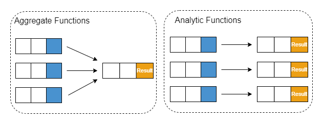
Analytic Functions
An analytic function (window function) performs an aggregate-like operation over a particular window (group of rows) but returns a single result for each row. OVER clause is commonly used with analytic functions to define that window.
Syntax
 <analytic_function> OVER (
    PARTITION BY <column>
    ORDER BY <column> ASC|DESC
    <window_frame>) <window_column_alias>
Parameters
<analytic_function> specifies the name of a function. For details, see the descriptions in Supported Functions following this discussion of Arguments.
OVER Clause
OVER clause is used to define the window specification with several parts, all optional:
PARTITION BY partitions rows into groups (partitions). The analytic function will be applied to each group. If not specified, the entire table is a partition. For example,
create table t(
    month MONTH,
    city STRING,
    sold INT
);

go

insert into t values(2023.06M, "A", 1200);
insert into t values(2023.07M, "A", 1500);
insert into t values(2023.08M, "B", 1200);
insert into t values(2023.07M, "B", 1300);
insert into t values(2023.07M, "C", 1300);
insert into t values(2023.06M, "C", 1400);
insert into t values(2023.08M, "A", 1400);
insert into t values(2023.06M, "B", 1000);
insert into t values(2023.08M, "C", 1100);

SELECT
  month,
  city,
  sum(sold) OVER (PARTITION BY city) AS sum
FROM t;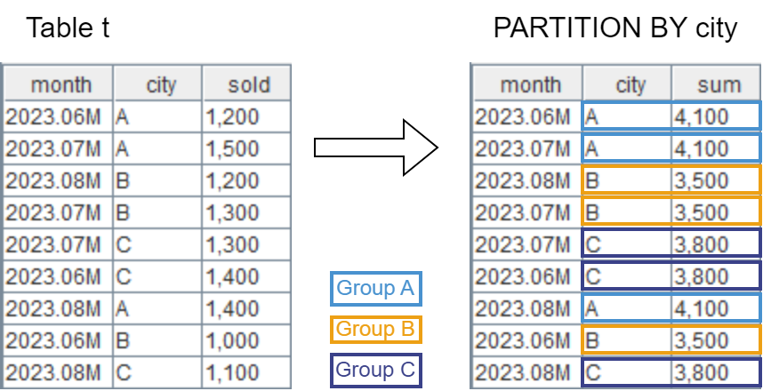
When applying the analytic function to a DFS table, if the PARTITION BY column is the partitioning column, the analytic function is executed within each partition; if not, the entire table will be loaded into memory and re-partitioned first before executing the analytic function.
ORDER BY orders rows within each partition into particular order before executing analytic functions. If ORDER BY is not specified, partition rows are unordered. Each ORDER BY clause optionally can be followed by ASC or DESC to indicate sort direction. The default is ASC. For example,
SELECT
  month,
  city,
  rank() OVER (PARTITION BY city ORDER BY month) AS rank
FROM t;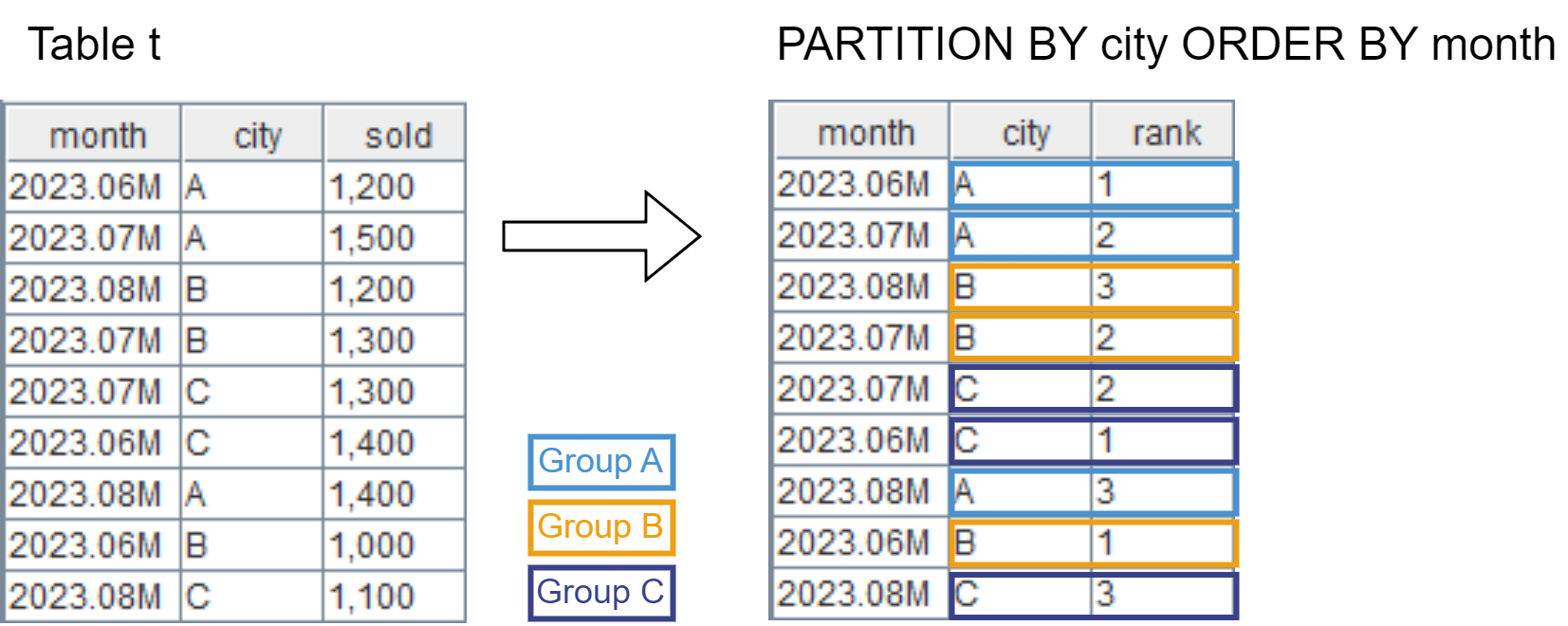
Based on the results of the above two examples, we can observe that the results preserve the order of the original table whether ORDER BY is specified or not.
<window_frame> is a subset of the current partition and it specifies which row to start the window on and where to end it. The range of the frame for a partition with r rows is within [1, r]. Analytic functions that operate on the entire partition should have no <window_frame>. Specifying <window_frame> is permitted for such functions but it will be ignored during execution.
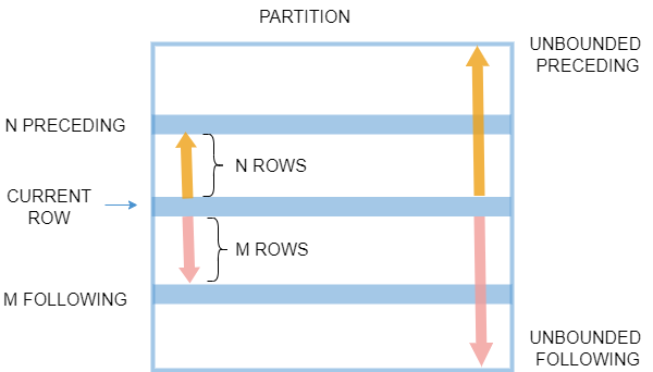
The <window_frame> clause, if given, has this syntax:
ROWS|RANGE BETWEEN lower_bound AND upper_bound-
ROWS and RANGE specifies how the frame is defined:
-
ROWS defines the frame by beginning and ending row positions.
-
RANGE defines the frame by rows within a range for the ORDER BY column. With RANGE set, ORDER BY clause must be specified and can only contain a single expression.
-
-
BETWEEN ... AND ... specifies the lower (starting) and upper (ending) boundary points of the window. lower_bound must not occur later than upper_bound. It can take the following values:
-
UNBOUNDED PRECEDING: The window starts at the first row of the partition.
-
n PRECEDING: For ROWS, the window starts n rows before the current row. For RANGE, the window starts at the row with values equal to the current row value minus n.
-
CURRENT ROW: The window begins or ends at the current row.
-
n FOLLOWING: For ROWS, the window ends n rows after the current row. For RANGE, the window ends at the row with values equal to the current row value plus n.
-
UNBOUNDED FOLLOWING: The window ends at the last row of the partition.
-
-
For ROWS, n must be a positive numeric integer.
-
For RANGE, n must be a positive numeric integer with the same unit as ORDER BY column, or a scalar of DURATION type with lower time precision than ORDER BY column. If both the n PRECEDING and n FOLLOWING options are set, the data type of n must be consistent.
Examples of the <window_frame> clause with BETWEEN…AND… keyword specified:
// The window starts at 1 row before the current row and ends 1 row after the current row.
ROWS BETWEEN 1 PRECEDING AND 1 FOLLOWING

// The window starts at the row with values equal to the current row value minus 200 and ends at the row with value equal to the current row value plus 100.
RANGE BETWEEN 200 PRECEDING AND 100 FOLLOWING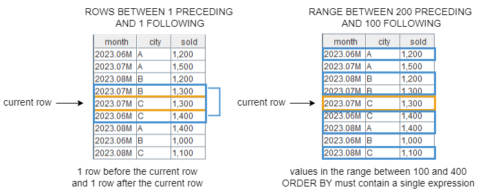
Where BETWEEN…AND… keyword is not specified, the frame is implicitly right-bounded by the current row.
-
ROWS | RANGE UNBOUNDED PRECEDINGis equal toROWS | RANGE BETWEEN UNBOUNDED PRECEDING AND CURRENT ROW. -
ROWS | RANGE n PRECEDINGis equal toROWS | RANGE BETWEEN n PRECEDING AND CURRENT ROW. -
ROWS | RANGE CURRENT ROWis equal toROWS | RANGE BETWEEN CURRENT ROW AND CURRENT ROW.
In the absence of a <window_frame> clause, the default frame depends on whether an ORDER BY clause is specified.
-
With ORDER BY, the default frame includes rows from the partition start through the current row, i.e.,
RANGE BETWEEN UNBOUNDED PRECEDING AND
                            CURRENT ROW
. -
Without ORDER BY, the default frame includes all partition rows, i.e.,
ROWS BETWEEN UNBOUNDED PRECEDING AND UNBOUNDED
                            FOLLOWING
.
Because the default frame differs depending on presence or absence of ORDER BY,
adding ORDER BY to a query may change the results. (For example, the values produced
by sum() might change.) To obtain the same results but ordered per
ORDER BY, it is recommended to specify a <window_frame> clause.
Note: When RANGE is specified, ORDER BY columns must be integral or time columns.
Supported Functions
Following are the supported functions for <analytic_function>. Note that the output results of the analytic function preserve the order of the original table.
|
Function |
Description |
|---|---|
| sum | Returns the sum. |
| sum2 | Returns the sum of squares. |
| avg | Returns the average value. |
| std | Returns the standard deviation. |
| stdp | Returns the population standard deviation. |
| var | Returns the standard variance. |
| varp | Returns the population standard variance. |
| count | Returns the row count. |
| min | Returns the minimum value. |
| imin | Returns the position of the element with the smallest value. If there are multiple identical minimum values, returns the position of the first minimum value starting from the left. |
| iminLast | Returns the position of the element with the smallest value. If there are multiple elements with the identical smallest value, returns the position of the first element from the right. |
| max | Returns the maximum value. |
| imax | Returns the position of the element with the largest value. If there are multiple identical maximum values, returns the position of the first maximum value starting from the left. |
| imaxLast | Returns the position of the element with the largest value. If there are multiple elements with the identical largest value, returns the position of the first element from the right. |
| skew | Returns the skewness. |
| kurtosis | Returns the kurtosis. |
| med | Returns the median. |
| row_number | Returns the sequential number of each row within the partition, starting at 1 for the first row. |
| rank | Returns the rank of each row within the partition. |
| dense_rank | Returns the rank of each row within the partition, with no gaps in the ranking values. |
| percent_rank | Returns the percent rank of a given row. The return value is within the range [0,1]. |
| cume_dist | Returns the cumulative distribution of a value within a group of values, i.e., the relative position of a specified value in a group of values. The return value is within the range (0,1]. |
| lead(expr, offset=1, default=NULL) | Returns the value of expr from the row that leads (follows) the current row by offset (optional) rows within its partition. If there is no such row, the return value is default (optional). <window_frame> is not supported. |
| lag(expr, offset=1, default=NULL) | Returns the value of expr from the row that lags (precedes) the current row by offset (optional) rows within its partition. If there is no such row, the return value is default (optional).<window_frame> is not supported. |
| ntile | Divides a partition into n groups, assigns each row in the partition its group number, and returns the number of the current row within its group. <window_frame> is not supported. |
| first_value | Returns the value of the first row within a partition of values. |
| last_value | Returns the value of the last row within a partition of values. |
| nth_value | Returns the value of the n-th row within a partition of values. |
| firstNot(X, [k]) | Returns the first element that is not null (or k). |
| lastNot(X, [k]) | Returns the last element that is not null (or k). |
| prod | Returns the product for all rows. |
| percentile(X, percent, [interpolation='linear']) | Returns the percentile of X. |
| wavg(X,Y) | Returns the weighted average of X with the weight vector Y. |
| wsum(X,Y) | Returns the inner product of X and Y. |
| corr(X, Y) | Returns the correlation of X and Y. |
| covar(X, Y) | Returns the covariance of X and Y. |
| beta(X, Y) | Returns the coefficient estimate of an ordinary-least-squares regression of Y on X. |
| atImax(location, value) | Finds the position of the element with the largest value in location, and returns the value of the element in the same position in value. |
| atImin(location, value) | Finds the position of the element with the smallest value in location, and returns the value of the element in the same position in value. |
Examples
The following is a sample table for examples 1-4.
create table t(
    id INT,
    sym SYMBOL,
    volume INT
);

insert into t values(1, `R, 200);
insert into t values(2, `P, 500);
insert into t values(1, `P, 100);
insert into t values(1, `P, 300);
insert into t values(2, `R, 300);
insert into t values(2, `P, 400);
insert into t values(3, `R, 400);

select * from t;| id | sym | volume |
|---|---|---|
| 1 | R | 200 |
| 2 | P | 500 |
| 1 | P | 100 |
| 1 | P | 300 |
| 2 | R | 300 |
| 2 | P | 400 |
| 3 | R | 400 |
Example 1: Specify <analytic_function> as an aggregate function.
Obtain the sum volume within the window frame (starts at 1 row before the current row and ends 2 rows after the current row) in each "sym" partition.
select
  *,
  sum(volume) over (
    partition by sym
    rows between 1 preceding and 2 following)
from
t;| id | sym | volume | sum |
|---|---|---|---|
| 1 | R | 200 | 900 |
| 2 | P | 500 | 900 |
| 1 | P | 100 | 1,300 |
| 1 | P | 300 | 800 |
| 2 | R | 300 | 900 |
| 2 | P | 400 | 700 |
| 3 | R | 400 | 700 |
Example 2: Specify <analytic_function> as a distribution function.
Obtain the percent rank of each "volume" row (in ascending order by default) in "sym" partition.
select
  *,
  percent_rank() over (
    partition by sym
    order by volume)
from
t;| id | sym | volume | percent_rank |
|---|---|---|---|
| 1 | R | 200 | 0 |
| 2 | P | 500 | 1 |
| 1 | P | 100 | 0 |
| 1 | P | 300 | 0.3333 |
| 2 | R | 300 | 0.5 |
| 2 | P | 400 | 0.6667 |
| 3 | R | 400 | 1 |
Example 3: Specify <analytic_function> as a ranking function.
Obtain the rank of each row within the "sym" partition.
// Without ORDER BY, ranks for all rows are the same.
select
  *,
  rank() over (
    partition by sym)
from
t;| id | sym | volume | rank |
|---|---|---|---|
| 1 | R | 200 | 1 |
| 2 | P | 500 | 1 |
| 1 | P | 100 | 1 |
| 1 | P | 300 | 1 |
| 2 | R | 300 | 1 |
| 2 | P | 400 | 1 |
| 3 | R | 400 | 1 |
// With ORDER BY, rank is applied on each "volume row" (in ascending order by default).
select
  *,
  rank() over (
    partition by sym
    order by volume)
from
t;| id | sym | volume | rank |
|---|---|---|---|
| 1 | R | 200 | 1 |
| 2 | P | 500 | 4 |
| 1 | P | 100 | 1 |
| 1 | P | 300 | 2 |
| 2 | R | 300 | 2 |
| 2 | P | 400 | 3 |
| 3 | R | 400 | 3 |
Example 4: Specify <analytic_function> as an analytic function.
Obtain the value of the first row within the window frame (starts at 2 rows before the current row and ends at the current row) in each "sym" partition.
 select
  *,
  first_value(volume) OVER(
    partition by sym
    ORDER BY id DESC
    rows 2 preceding)
from
t;| id | sym | volume | first_value |
|---|---|---|---|
| 1 | R | 200 | 400 |
| 2 | P | 500 | 500 |
| 1 | P | 100 | 500 |
| 1 | P | 300 | 400 |
| 2 | R | 300 | 400 |
| 2 | P | 400 | 500 |
| 3 | R | 400 | 400 |
Example 5: Query for a DFS table using analytic function.
t = table(1 2 1 1 2 2 3 as id, `R`P`L`P`R`L`R as sym, 200 500 100 300 300 400 400 as volume)
db_name = "dfs://window_function"
if (existsDatabase(db_name)) {
    dropDatabase(db_name)
}
db = database(db_name, HASH, [INT, 2], , 'TSDB')

pt = db.createPartitionedTable(t, "pt", "id", ,"volume")
pt.append!(t)

// Obtain the value of "volume" from the row that leads the current row by 1 row within each "sym" partition where the "id" is sorted in ascending order. If there is no such row, the return value is -1.
select
  *,
  lead(volume, 1, -1) OVER(
    PARTITION BY sym
    ORDER BY id)
from
t;| id | sym | volume | lead |
|---|---|---|---|
| 1 | R | 200 | 300 |
| 2 | P | 500 | -1 |
| 1 | L | 100 | 400 |
| 1 | P | 300 | 500 |
| 2 | R | 300 | 400 |
| 2 | L | 400 | -1 |
| 3 | R | 400 | -1 |
Example 6: Specify <window_frame> as a time range by using the RANGE keyword with n as a scalar of the DURATION data type.
n=10
date= rand(2022.10.01..2022.10.04 join 2022.11.01 join 2022.12.04 join 2022.12.06 join 2022.12.10 join 2023.01.01 join 2023.02.02, n)
price = [49.6,29.46,49.6,50.6,64.97,56.9,50.66,50.32,51.29,62.36]
qty = [2200,1900,2000,2200,6800,2100,1300,6600,8800,5300]
sym = rand(string(["C", "MS", "A"]), n)
t = table(date, sym, qty, price);
t| date | sym | qty | price |
|---|---|---|---|
| 2022.10.02 | C | 2,200 | 49.6 |
| 2022.12.06 | C | 1,900 | 29.46 |
| 2022.12.10 | C | 2,000 | 49.6 |
| 2022.10.02 | A | 2,200 | 50.6 |
| 2022.10.02 | MS | 6,800 | 64.97 |
| 2023.02.02 | C | 2,100 | 56.9 |
| 2022.10.01 | C | 1,300 | 50.66 |
| 2023.02.02 | MS | 6,600 | 50.32 |
| 2022.10.03 | A | 8,800 | 51.29 |
| 2022.12.04 | MS | 5,300 | 62.36 |
Obtain the maximum value of "qty" within the window frame (starts at 1 month before the current date and ends 1 month after the current date) in each "sym" partition.
select *, max(qty) over (partition by sym order by date RANGE BETWEEN 1M PRECEDING AND 1M FOLLOWING) from t| date | sym | qty | price | max |
|---|---|---|---|---|
| 2022.10.02 | C | 2,200 | 49.6 | 2,200 |
| 2022.12.06 | C | 1,900 | 29.46 | 2,000 |
| 2022.12.10 | C | 2,000 | 49.6 | 2,000 |
| 2022.10.02 | A | 2,200 | 50.6 | 8,800 |
| 2022.10.02 | MS | 6,800 | 64.97 | 6,800 |
| 2023.02.02 | C | 2,100 | 56.9 | 2,100 |
| 2022.10.01 | C | 1,300 | 50.66 | 2,200 |
| 2023.02.02 | MS | 6,600 | 50.32 | 6,600 |
| 2022.10.03 | A | 8,800 | 51.29 | 8,800 |
| 2022.12.04 | MS | 5,300 | 62.36 | 5,300 |