Quick Examples

The bid-ask spread is defined as the difference between the best offer price (offerPrice0) and best bid price (bidPrice0) divided by the average price, with the formula as follows:

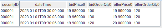
An example of the input data is as shown below.

(1) Create a shared stream table tick as the publishing table:

share(table=streamTable(1:0, `securityID`dateTime`bidPrice0`bidOrderQty0`offerPrice0`offerOrderQty0, [SYMBOL,TIMESTAMP,DOUBLE,LONG,DOUBLE,LONG]), sharedName=`tick)

(2) Create a shared stream table resultTable to store calculation results:

share(table=streamTable(1:0, ["securityID", "dateTime", "factor"], [SYMBOL, TIMESTAMP, DOUBLE]), sharedName=`resultTable)

Subsequent calculation results will be written to this table in real time.

(3) Define the factor calculation function factorCalFunc to compute the bid-ask spread factor for each stock:

def factorCalFunc(msg){
	tmp = select securityID, dateTime, (offerPrice0-bidPrice0)*2\(offerPrice0+bidPrice0) as factor from msg
	objByName("resultTable").append!(tmp)	
}

• msg is an in-memory table with the same schema as the tick table.
• objByName("resultTable").append!(tmp) appends the calculation results in the temporary table tmp to the result table resultTable.
• The temporary table tmp is generated using DolphinDB SQL statements. The formula (offerPrice0-bidPrice0)*2/(offerPrice0+bidPrice0) calculates the bid-ask spread factor for each row in the msg table.

(4) Subscribe to the stream table tick and specify the computation logic:

subscribeTable(tableName="tick", actionName="factorCal", offset=-1, handler=factorCalFunc, msgAsTable=true, batchSize=1, throttle=0.001)

The subscription task processes incoming data with UDF factorCalFunc (where bid-ask spread is defined) and outputs results to resultTable each time new record is inserted into the tick table.

• tableName="tick" indicates that the subscription is for the stream table tick.
• actionName="factorCal" specifies a unique name for the subscription task.
• offset=-1 means processing starts from the first arrived message after subscription.
• handler=factorCalFunc specifies that the factorCalFunc function is used to process the data.
• msgAsTable=true indicates that the subscribed data is input as a table to the function factorCalFunc.
• batchSize=1 control the processing frequency, triggering computation whenever a new record arrives.

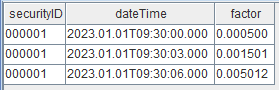
(5) Then inject simulated data to the stream table tick to observe the processing results:

insert into tick values(`000001, 2023.01.01T09:30:00.000, 19.98, 100, 19.99, 120)
insert into tick values(`000001, 2023.01.01T09:30:03.000, 19.96, 130, 19.99, 120)
insert into tick values(`000001, 2023.01.01T09:30:06.000, 19.90, 120, 20.00, 130)

After inserting these rows into the tick table, the resultTable will automatically update with the computed factor values.

The active buy volume ratio is the ratio of active buy volume to total trade volume, calculated as follows:

where actVolume_t represents the active buy volume within the interval from t-window to t, and totalVolume_t represents the total trade volume within the same interval.

The signal function I is defined as follows:

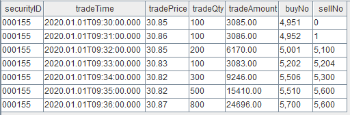
An example of the input data is as shown below.

(1) Create a shared stream table trade as the publishing table:

share(table=streamTable(1:0, `securityID`tradeTime`tradePrice`tradeQty`tradeAmount`buyNo`sellNo, [SYMBOL,TIMESTAMP,DOUBLE,INT,DOUBLE,LONG,LONG]), sharedName=`trade)

(2) Create a shared stream table resultTable to store calculation results:

share(table=streamTable(1:0, ["securityID", "tradeTime", "factor"], [SYMBOL, TIMESTAMP, DOUBLE]), sharedName=`resultTable) 

Subsequent calculation results will be written to this table in real time.

(3) Define the factor calculation function.

The active buy volume ratio is calculated by looking back over a 5-minute window based on the current record and aggregating data within that window. As the input streams continue to grow, the window slides forward in real time. Different from the bid-ask spread calculation, this case requires both the latest input record and historical data within a certain timeframe. This section first introduces an incorrect implementation to illustrate potential issues with stateless calculations, followed by the correct approach.

Incorrect Implementation

Define a function factorVolumeCalFunc:

def factorVolumeCalFunc (msg){
	tmp = select securityID, tradeTime, tmsum(tradeTime, iif(buyNo>sellNo, tradeQty, 0), 5m)\tmsum(tradeTime, tradeQty, 5m) as factor from msg context by securityID
	objByName("resultTable").append!(tmp)
}
subscribeTable(tableName="trade", actionName="factorCal", offset=-1, handler=factorVolumeCalFunc , msgAsTable=true, batchSize=1, throttle=0.001)

• msg is an in-memory table with the same schema as the tick table.
• objByName("resultTable").append!(tmp) appends the calculation results in the temporary table tmp to the result table resultTable.
• The temporary table tmp is generated using DolphinDB SQL statements:
  • context by securityID groups msg by securityID.
  • tmsum(tradeTime, tradeQty, 5m) computes the trading volume in the past 5 minutes based on the tradeTime column.
  • tmsum(tradeTime, iif(buyNo>sellNo, tradeQty, 0), 5m) computes the active trading volume for records (with buyNo>sellNo) in the past 5 minutes.

We use simulated data to observe the results:

share(table=streamTable(10000:0, ["securityID", "tradeTime", "factor"], [SYMBOL, TIMESTAMP, DOUBLE]), sharedName=`resultTable)
// Ingest simulated data
input1 = table(1:0, `securityID`tradeTime`tradePrice`tradeQty`tradeAmount`buyNo`sellNo, [SYMBOL,TIMESTAMP,DOUBLE,INT,DOUBLE,LONG,LONG])
insert into input1 values(`000155, 2020.01.01T09:30:00.000, 30.85, 100, 3085, 4951, 0)
insert into input1 values(`000155, 2020.01.01T09:31:00.000, 30.86, 100, 3086, 4952, 1)
insert into input1 values(`000155, 2020.01.01T09:32:00.000, 30.85, 200, 6170, 5001, 5100)
insert into input1 values(`000155, 2020.01.01T09:33:00.000, 30.83, 100, 3083, 5202, 5204)
insert into input1 values(`000155, 2020.01.01T09:34:00.000, 30.82, 300, 9246, 5506, 5300)
insert into input1 values(`000155, 2020.01.01T09:35:00.000, 30.82, 500, 15410, 5510, 5600)
insert into input1 values(`000155, 2020.01.01T09:36:00.000, 30.87, 800, 24696, 5700, 5600)
// Call factorVolumeCalFunc
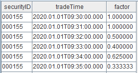
factorVolumeCalFunc(msg=input1)

Check resultTable:

select * from resultTable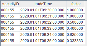

Then ingest another record and call the function again:

input2 = table(1:0, `securityID`tradeTime`tradePrice`tradeQty`tradeAmount`buyNo`sellNo, [SYMBOL,TIMESTAMP,DOUBLE,INT,DOUBLE,LONG,LONG])
insert into input2 values(`000155, 2020.01.01T09:36:00.000, 30.87, 800, 24696, 5700, 5600)
factorVolumeCalFunc (msg=input2)

The latest result is incorrect.

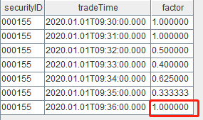
This approach calculates based only on new records in the trade table without caching or retrieving necessary historical data, leading to incorrect results.

Correct Implementation

createReactiveStateEngine(name="reactiveDemo", metrics=<[tradeTime, tmsum(tradeTime, iif(buyNo>sellNo, tradeQty, 0), 5m)\tmsum(tradeTime, tradeQty, 5m)]>, dummyTable=trade, outputTable=resultTable, keyColumn="securityID")
def factorVolumeCalFunc (msg){
    getStreamEngine("reactiveDemo").append!(msg)
}

• name="reactiveDemo" specifies the unique name for the engine.
• dummyTable=trade specifies that the input table schema matches the trade table.
• outputTable=resultTable indicates the results will be output to resultTable.
• keyColumn="securityID" groups data by securityID. Each group maintains its state independently.
• metrics defines the calculation logic, where
  • tradeTime outputs the tradeTime column from input data.
  • tmsum(tradeTime, iif(buyNo > sellNo, tradeQty, 0), 5m) computes active trading volume over the past 5 minutes.
  • tmsum(tradeTime, tradeQty, 5m) computes total trading volume over the past 5 minutes.

In the reactive state engine, moving functions like tmsum are incrementally computed based on previous results, caching necessary states for efficiency. For example, the total trade volume can be updated following the incremental computation logic: Total Volume(t) = Total Volume(t-1) + Current Volume - Expired Volume.

(4) Subscribe to the table trade to ingest the data to a reactive state engine. The metrics of the engine define how to calculate active buy volume ratio with tmsum function (which is incrementally optimized within the engine).

createReactiveStateEngine(name="reactiveDemo", metrics=<[tradeTime, tmsum(tradeTime, iif(buyNo>sellNo, tradeQty, 0), 5m)\tmsum(tradeTime, tradeQty, 5m)]>, dummyTable=trade, outputTable=resultTable, keyColumn="securityID")
subscribeTable(tableName="trade", actionName="factorCal", offset=-1, handler=getStreamEngine("reactiveDemo"), msgAsTable=true, batchSize=1, throttle=0.001)

insert into trade values(`000155, 2020.01.01T09:30:00.000, 30.85, 100, 3085, 4951, 0)
insert into trade values(`000155, 2020.01.01T09:31:00.000, 30.86, 100, 3086, 4952, 1)
insert into trade values(`000155, 2020.01.01T09:32:00.000, 30.85, 200, 6170, 5001, 5100)
insert into trade values(`000155, 2020.01.01T09:33:00.000, 30.83, 100, 3083, 5202, 5204)
insert into trade values(`000155, 2020.01.01T09:34:00.000, 30.82, 300, 9246, 5506, 5300)
insert into trade values(`000155, 2020.01.01T09:35:00.000, 30.82, 500, 15410, 5510, 5600)

Check resultTable:

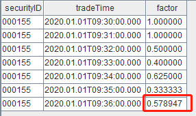
Then ingest another record:

insert into trade values(`000155, 2020.01.01T09:36:00.000, 30.87, 800, 24696, 5700, 5600)

The result for 09:36:00 is as expected.

Use the unsubscribeTable function to cancel a specific subscription:

unsubscribeTable(tableName="trade", actionName="factorCal")

Use the dropStreamEngine function to release the streaming engine and free the memory:

dropStreamEngine(`reactiveDemo)

Use the undef function to delete shared stream tables:

dropStreamTable(`trade)