Backtesting Application: Medium- and High-Frequency Options Spread Strategy with Volatility Timing

In today’s highly sophisticated derivatives markets, options and their combination strategies have become essential tools for institutional investors to conduct refined risk management and generate alpha. Implied volatility (IV), a core parameter in option pricing, often exhibits short-term fluctuations that create abundant trading opportunities. By constructing multi-leg option portfolios, traders can capture volatility-driven returns while limiting directional exposure.

Before deploying complex strategies involving multi-leg structures, high-frequency signal generation, and dynamic risk control into live trading, it is crucial to conduct rigorous and efficient backtesting using high-quality historical data to evaluate their robustness and feasibility. Leveraging its high-performance computing engine and powerful data processing capabilities, DolphinDB provides an ideal platform for medium- and high-frequency quantitative strategy backtesting. In this article, we demonstrate how to implement a full backtesting workflow using DolphinDB’s backtest plugin for a volatility-timed vertical spread strategy with option snapshot data.

An option is a financial contract that grants the buyer the right, but not the obligation, to buy or sell an underlying asset at a specified price on or before a given date. The price of an option is primarily influenced by several factors: the current price of the underlying asset (S0), the strike price (K), time to maturity (T), the expected future volatility of the underlying (σ), and the risk-free interest rate (r). Among these factors, future volatility (σ) is the only unobservable variable, making it the central component of option pricing and trading. In practice, pricing models such as the Black-Scholes-Merton (BSM) model are commonly used to infer implied volatility from market option prices, reflecting the market’s consensus expectation of future volatility.

In trading practice, volatility traders often construct delta-neutral portfolios to profit from mispricing or relative changes in implied volatility. For instance, when implied volatility is expected to rise, traders may establish positive vega positions such as long straddles. Conversely, when implied volatility is expected to decline, negative vega portfolios can be constructed to benefit from volatility compression.

Implied volatility can also serve as an important timing factor in directional option strategies. For example, if the market outlook on the underlying asset is moderately bullish and implied volatility is relatively low, traders may adopt a bull call spread. This allows them to gain directional exposure at a relatively low cost while limiting downside risk. Conversely, when the outlook turns moderately bearish and implied volatility is relatively high, a bear put spread can be employed to establish short exposure while keeping potential losses from upward price movements under control.

Building on this idea, we implement a vertical spread strategy that incorporates volatility timing signals . The strategy determines directional exposure based on the forecast of the underlying asset price and dynamically selects between a bull call spread and a bear put spread depending on the current implied volatility regime.

A typical medium- and high-frequency quantitative backtesting platform consists of three core components: market data replay, order matching simulation, and strategy execution with performance evaluation. However, implementing such systems presents several challenges:

Massive high-frequency datasets impose stringent requirements on query and computation performance.
The backtesting environment should closely simulate market conditions, including order execution probability, transaction prices, trading volume, and market impact.
The system architecture must be flexible and extensible to support diverse strategies and technical indicators.

To address these challenges, DolphinDB provides a high-performance and scalable backtesting framework based on its distributed storage and computing architecture. The solution consists of three critical components:

Market Data Replay

The replay feature streams historical data from one or more distributed tables into stream tables in strict chronological order or according to specified sorting rules. This provides a unified environment for both research and production, enabling real-time factor computation on historical data.

Matching Engine Simulator Plugin

The plugin supports both Level-2 tick-by-tick data and snapshot data. It follows the price-time priority matching rule and provides high-precision order execution simulation. Multiple matching modes and flexible parameter configurations are available to better emulate live trading environment.

Backtesting Framework

The backtesting framework allows users to define custom indicators and supports strategy evaluation based on tick-level, snapshot-level, minute-level, or daily data. It outputs comprehensive results including returns, positions, and detailed trade records. High-precision backtesting based on tick or snapshot data enables integrated validation of both simulation and historical backtests.

The solution’s modular structure allows for seamless integration with existing systems, accommodating users who may already deploy certain components in place. This adaptability enables traders to construct a comprehensive backtesting system from the ground up using DolphinDB's full suite of tools, or enhance their current setup by incorporating specific DolphinDB capabilities.

1. Option Volatility-Timing Spread Strategy Based on DolphinDB

1.1 Strategy Logic

In this article, we implement a volatility-timing options spread strategy on gold options using full intraday data from the Shanghai Futures Exchange (SHFE) and the DolphinDB Backtest plugin. The strategy logic is summarized below:


Strategy Parameter	Value
Start date	2025-02-17 (Intraday start)
End date	2025-02-17 (Intraday end)
Backtest frequency	Snapshot-level
Initial capital	1,000,000
Underlying	Call & Put options for the main gold futures contract
Entry signals	Bull call spread Entry Signal (IV low & underlying price uptrend) Current option IV < 30-snapshot IV mean - 1.0 * standard deviation(σ) Latest futures price MACD > 0, and previous snapshot MACD < 0 Bear put spread entry signal (IV high & underlying price downtrend) Current option IV > 30-snapshot IV mean + 1σ Latest futures price MACD < 0, and previous snapshot MACD > 0
Position construction	Positions are established in real time according to IV signals: Bull call spread: long an at-the-money (ATM) call + short a call two strikes OTM. Bear put spread: long an ATM put + short a put two strikes OTM.
Exit signals	The spread between the ATM and OTM option legs is monitored in real time for each option spread. For both bull call and bear put spreads, a widening ATM–OTM spread indicates increasing profit. Positions are closed with market orders when the relative change in the spread from its initial level reaches the predefined bounds of [-3%, 5%], where Relative change = (current spread − initial spread) / initial spread.

1.2 Profit and Loss (P&L) Scenarios

We analyze the profit and loss of the option spreads used in the current strategy. Assume that the underlying gold futures price is 675 CNY/g. The corresponding ATM and two strikes OTM options for both the call and put directions, along with their opening premiums, are shown below.


Option Type	Symbol	Premium Paid/Received to Open
An ATM call option	AU2503-C-672	C1
A call option two strikes OTM	AU2503-C-688	C2
An ATM put option	AU2503-P-672	C3
A put option two strikes OTM	AU2503-P-656	C4

Note: Since the premium of an ATM option is higher than that of an OTM option, we have C1 > C2 and C3 > C4.

1.2.1 Bull Call Spread Option Position

Assume that IV is relatively low and the underlying futures price is trending upward, triggering a bull call spread signal—that is, buying an ATM call option and selling a call option two strikes OTM.

The underlying gold futures price (St) may evolve under the following three scenarios:

Significant decline (St << 672)
Moderate increase or sideways movement (672 ≤ St ≤ 688)
Significant increase (St >> 688)

For each of these scenarios, the P&L direction and magnitude of the ATM call, the call option two strikes OTM, and the overall option spread are summarized in the table below.


Gold Futures	ATM Call Option (Long)	Call Option Two Strikes OTM (Short)	Bull Call Spread (1:1)
Significant Decline	Large floating loss, option value decays rapidly P&L: -C1	Large floating profit, option value decays rapidly P&L: +C2	Floating loss, reaching maximum loss, spread narrows sharply P&L is -(C1 - C2)
Moderate Increase / Sideways	Floating profit: the ATM call typically has a positive delta, so its price increases as the underlying rises, generating gains for the long position. P&L: > -C1	Floating loss: the option has a positive delta, so its price increases as the underlying rises, leading to losses for the short leg. P&L: < +C2	The ATM option typically has a larger absolute delta than the OTM option, resulting in a net positive delta for the spread. When the underlying price rises, the ATM–OTM spread widens, generating floating profit. When the underlying price falls, the spread narrows, resulting in floating loss.
Significant Increase	Deep ITM: the long ATM call increases rapidly in value as the underlying price rises, generating floating profit for the long position. P&L: (St - 672) - C1	Deep ITM: the short OTM call gains value rapidly as the underlying price rises, resulting in increasing losses for the short leg. P&L: (St - 688) + C2	The ATM–OTM call spread widens to its maximum extent, producing the maximum floating profit for the position. P&L: (688 - 672) - (C1 - C2)

1.2.2 Bear Put Spread Option Position

Assume that IV is relatively high and the underlying futures price is trending downward, triggering a bear put spread signal—that is, buying an ATM put option and selling a put option two strikes OTM.

The underlying gold futures price (St) may evolve under the following three scenarios:

Significant decline (St<<656)
Moderate decrease or sideways movement (656≤St≤672)
Significant increase (St>>672)

For each of these scenarios, the P&L direction and magnitude of the ATM put, the put option two strikes OTM, and the overall option spread are summarized in the table below.


Gold Futures	ATM Put Option (Long)	Put Option Two Strikes OTM (Short)	Bear Put Spread (1:1)
Significant Decline	Deep ITM: the long ATM put increases rapidly in value as the underlying price falls, generating floating profit for the long position. P&L: (672 - St) - C3	Deep ITM: the short OTM put loses value rapidly as the underlying price falls, resulting in increasing losses for the short leg. P&L: (St - 656) + C4	The ATM–OTM put spread widens to its maximum extent, producing the maximum floating profit for the position. P&L: (672 - 656) -(C3 - C4)
Moderate Decrease / Sideways	Floating profit: the ATM put typically has a negative delta, so its price increases as the underlying price falls, generating gains for the long position. P&L: > - C3	Floating loss: the OTM put typically has a negative delta, so its price decreases as the underlying rises, leading to losses for the short leg. P&L: < +C4	The ATM option typically has a larger absolute delta than the OTM option, resulting in a net negative delta for the spread. When the underlying price falls, the ATM–OTM spread widens, generating floating profit. When the underlying price rises, the spread narrows, resulting in floating loss.
Significant Increase	Large floating loss: the ATM put loses value rapidly as the underlying price rises. P&L: -C3	Large Floating profit: the OTM put gains value rapidly as the underlying price rises. P&L: +C4	The ATM–OTM put spread narrows sharply, reaching maximum floating loss for the position. P&L: -(C3 - C4)

1.2.3 P&L Summary

Both the bull call spread and bear put spread collect premium from selling options to offset the cost of buying the other leg. This strategy has two key characteristics:

Limited maximum loss: the total potential loss of the spread is capped at the initial net expenditure when the underlying moves in an adverse direction.
Limited maximum profit: the total profit is capped at the difference between strike prices minus the net premium paid.

By sacrificing unlimited upside potential, the strategy significantly lowers the breakeven point and reduces the required margin for hedging.

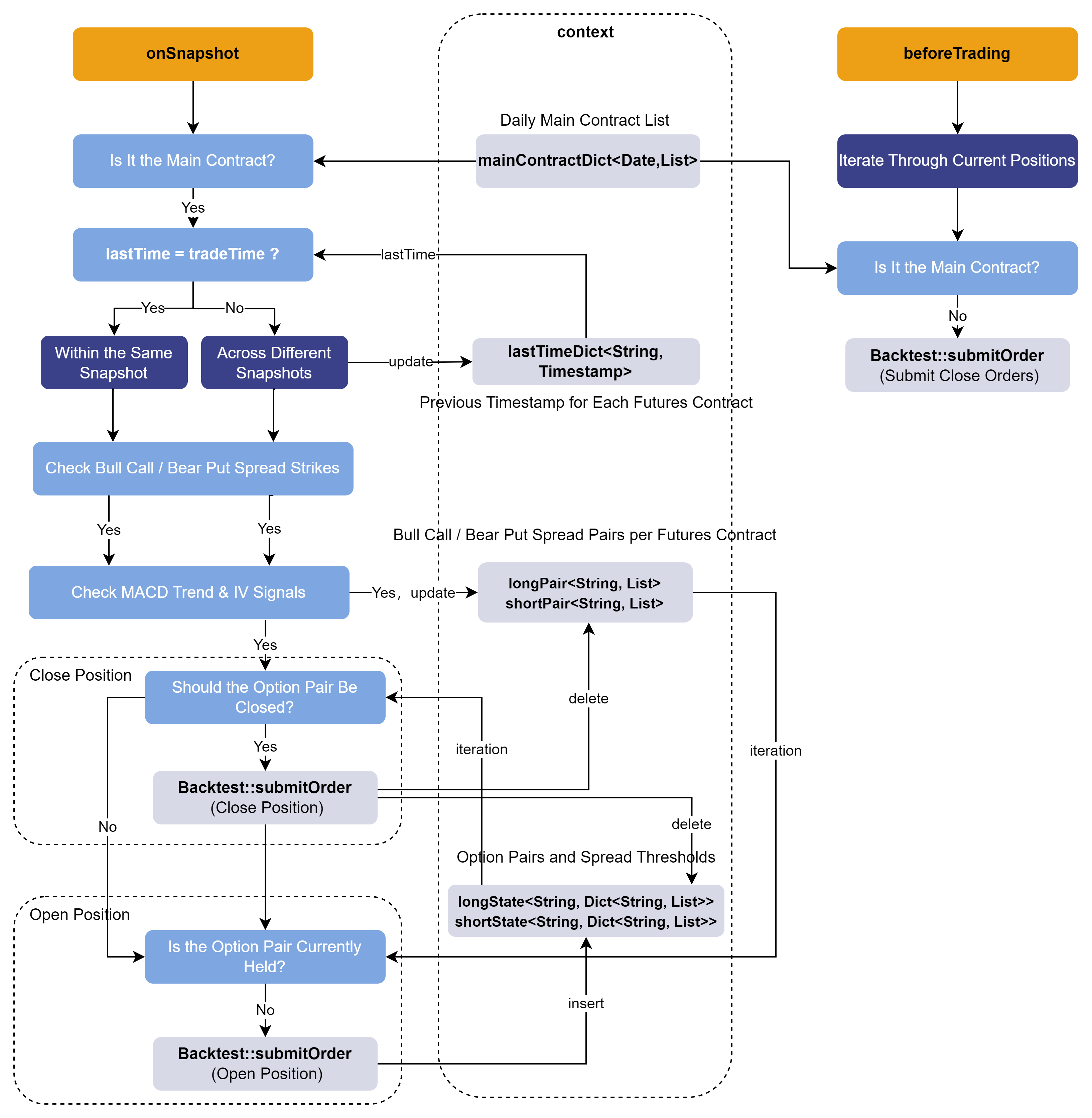
1.3 Strategy Structure

The DolphinDB Backtest plugin provides a variety of event-driven callback functions, including onSnapshot , onBar , and onTrade . The onSnapshot callback is primarily used to implement the intraday option volatility-timing spread strategy at snapshot frequency, in conjunction with the context state of the DolphinDB Backtest plugin.

Within the context state, three types of variables are defined for the strategy:

lastTimeDict – stores the previous timestamp for each futures contract.
longPair and shortPair – represent the bull call spread and bear put spread option pairs for each futures contract, respectively.
longState and shortState – record the corresponding option pairs and the configured spread bounds for the bull call spread and bear put spread positions.

The overall implementation logic of the strategy is summarized as follows:

Figure 1. Figure 1-1 Snapshot-Frequency Option Volatility-Timing Spread Strategy

1.3.1 Retrieving Basic Information

Within the onSnapshot callback, three input parameters are provided sequentially:

context: a dictionary to restore the context state.
msg: a dictionary to restore the snapshot market data.
indicator: the custom indicator object.

First, option contract information is collected, including the option symbol, the corresponding futures contract, option type (call/put), and strike price levels. Then, the list of the day’s main contract is obtained, and market data for non-main contracts is excluded.

def onSnapshot(mutable contextInfo, msg, indicator){
    /* Snapshot callback
    msg structure: a dictionary containing the data of an instrument in the snapshot
    symbol-> 
    symbolSource->    
    ...
    indicator: a dictionary containing the computed indicators of the instrument
    ...
    */
    // Get instrument-level option information
    ioption = msg.symbol                                // Option symbol
    direction = contextInfo["directionDict"][ioption]   // Call (1) or Put (2)
    contract = contextInfo["contractDict"][ioption]    // Underlying futures contract 
    strike = contextInfo["strikePriceDict"][ioption]    // Option strike price
    // Get the signal information
    level = msg["signal"][0]                            // Option strike price levels
    ivSignal = msg["signal"][1]                         // Options IV signal
    trendSignal = msg["signal"][2]                      // Futures price MACD trend signal
    // Get current time information
    tradeTime = contextInfo["tradeTime"]
    tradeDate = contextInfo["tradeDate"]
    // Filter out non-main contracts
    contractList = contextInfo["mainContractDict"][tradeDate] // Today's main contract list
    if (!(contract in contractList)){ // Non-main contract
        return
    }
    ...
}

1.3.2 Selecting Option Pairs

Since the latest price of the underlying futures changes in real time, it is necessary to continuously track the strike price levels of the target options. To support multi-symbol and multi-contract scalability in the strategy, a nested dictionary with the structure <STRING, Dict<STRING, VECTOR>> is used as a state variable. The outer STRING indicates the futures contract symbol, the inner STRING indicates the option pair name, and the VECTOR is a two-element string vector corresponding to [ATM option symbol, two-strike OTM symbol] . The two options within the vector form an option pair, and the corresponding order logic is executed for each pair during the subsequent position-opening process.

In the onSnapshot callback, the target option pairs are selected in real time as follows:

All options are evaluated, and if an option is in the bull call spread direction (i.e., the ATM call and the call option two strikes OTM), it is placed into the longPair state variable; Otherwise, if it is in the bear put spread direction (i.e., the ATM put and the put option two strikes OTM), it is placed into the shortPair state variable.
During the subsequent opening logic, positions are established based on the option pairs stored in longPair and shortPair.

ivSignal = msg["signal"][1]  // ivFactor
trendSignal = msg["signal"][2] // trendFactor
// Bull Call / Bear Put signals -> add to longPair & shortPair
if (ivSignal == 1 and trendSignal == 1){
    // Bull Call signal triggered -> long ATM call + short call option two strikes OTM
    if (!(contract in keys(contextInfo["longPair"]))){
        contextInfo["longPair"][contract] = array(STRING, 2)
    }
    if (level == 0 and direction == 1){ // ATM call
        contextInfo["longPair"][contract][0] = ioption
    }else if (level == -2 and direction == 1){ // Call option two strikes OTM
        contextInfo["longPair"][contract][1] = ioption
    }
}else if (ivSignal == -1 and trendSignal == -1){ 
    // Bear Put signal triggered -> long ATM put + short put two strikes OTM
    if (!(contract in keys(contextInfo["shortPair"]))){
        contextInfo["shortPair"][contract] = array(STRING, 2)
    }
    if (level == 0 and direction == 2){ // ATM put
        contextInfo["shortPair"][contract][0] = ioption
    }else if (level == -2 and direction == 2){ // Put two strikes OTM
        contextInfo["shortPair"][contract][1] = ioption
    }
}

1.3.3 Constructing Cross-Sectional Order Execution

The onSnapshot callback is triggered once for each snapshot of each instrument. Cross-sectional snapshots can be constructed by aligning snapshots across instruments based on their timestamps, enabling the implementation of cross-sectional order execution. Since the ingested data is already sorted by timestamp, the tradeTime for each contract in the callback is guaranteed to be monotonically increasing, so this logic is valid.

The code for constructing cross-sectional snapshots within the onSnapshot callback is as follows: for different options within a single futures contract snapshot, the callback can terminate immediately; only when the current timestamp differs from the previous one—that is, when moving to the next cross-sectional snapshot for a futures contract—should the corresponding state variables be retrieved from the context to perform position closing and opening, after which the remaining code logic continues to execute.

// Get current time information
... // Code block applied to all underlyings
tradeTime = contextInfo["tradeTime"]
if (contextInfo["lastTimeDict"][contract]==tradeTime){
    return 
}else{ // Next snapshot section
    contextInfo["lastTimeDict"][contract]=tradeTime.copy()
}
... // Code block triggered only on snapshot change

1.3.4 Closing Option Pair Positions

Based on the analysis in Section 2.1, the spread between the ATM and OTM options plays a crucial role in the final P&L of the option spreads constructed. Therefore, it is necessary to track the changes in the spread in real time and close the option pairs at the appropriate time.

The code segment for closing positions is shown below (taking the Bull Call Spread option pair as an example):

if (contract in keys(contextInfo["longState"])){  
   // longState stores [long ATM call, short call option two strikes OTM] -> Closing logic [Close Long, Close Short]
    for (optPair in keys(contextInfo["longState"][contract])){
        opt1 = optPair.split("$")[0]    // ATM Call
        opt2 = optPair.split("$")[1]    // Call option two strikes OTM
        price1 = contextInfo["lastPriceDict"][opt1]
        price2 = contextInfo["lastPriceDict"][opt2]
        state = price1 - price2 // Compute latest spread
        stateList = contextInfo["longState"][contract][optPair] // Min & Max spread
        // Check if spread breaks threshold
        if (state<stateList[0] or state>stateList[1]){
            vol1 = Backtest::getPosition(contextInfo["engine"], symbol=opt1)["longPosition"][0]  
            // ATM Call long
            vol2 = Backtest::getPosition(contextInfo["engine"], symbol=opt2)["shortPosition"][0] 
            // OTM Call short
            if (isNull(vol1) or isNull(vol2)){
                continue
            }
            if (vol1>0 and vol2>0){
                orderDirection = 3 // Close long
                Backtest::submitOrder(contextInfo["engine"],
                    (opt1, "SHFE", tradeTime, 0, price1, price1, vol1, orderDirection, 0),
                    label="closeLong",orderType=0)
                orderDirection = 4 // close short
                Backtest::submitOrder(contextInfo["engine"],
                    (opt2, "SHFE", tradeTime, 0, price2, price2, vol2, orderDirection, 0),
                    label="closeShort",orderType=0)
                // Remove spread record
                contextInfo["longState"][contract].erase!(opt1+"$"+opt2)
                contextInfo["longPair"] = array(STRING, 2)
            }
        }
    }
}

1.3.5 Opening Option Pair Positions

For the opening logic, the Backtest::getAvailableCash function is used to check the real-time available cash, preventing orders from being placed when funds are insufficient. Next, orders are executed based on the bull call spread and bear put spread option pairs stored in longPair and shortPair, respectively.

Note that to avoid duplicate orders, the Backtest::getPosition function is used to retrieve the current positions of the underlying and check whether there are existing positions in the corresponding direction.

The code segment for opening positions is shown below (taking the bull call spread option pair as an example):

if (Backtest::getAvailableCash(contextInfo["engine"]) <= 100000){
    return 
}
// Bull call spread → long ATM call + short call option two strikes OTM
if (contract in keys(contextInfo["longPair"])){
    opt1 = contextInfo["longPair"][contract][0]
    opt2 = contextInfo["longPair"][contract][1]
    vol1 = Backtest::getPosition(contextInfo["engine"], symbol=opt1)["longPosition"][0]
    vol2 = Backtest::getPosition(contextInfo["engine"], symbol=opt2)["shortPosition"][0]
    price1 = contextInfo["lastPriceDict"][opt1]
    price2 = contextInfo["lastPriceDict"][opt2]
    optPair = opt1+"$"+opt2
    if (!isNull(opt1) and !isNull(opt2) and price1!=price2){  // Initial spread is not zero
        // Check if current option is already held
        state = false
        if (!(isNull(vol1))){
            if (vol1 >0){
                state = true
            }
        }
        if (!(isNull(vol2))){
            if (vol2 >0){
                state = true
            }
        }
        if (!state){
            // Open 1 lot
            orderDirection = 1 // ATM Call long
            Backtest::submitOrder(contextInfo["engine"],
                (opt1, "SHFE", tradeTime, 0, price1, price1, 1, orderDirection, 0),
                label="openLong",orderType=0) // Order (0: Market)
            orderDirection = 2 // Short call option two strikes OTM
            Backtest::submitOrder(contextInfo["engine"],
                (opt2, "SHFE", tradeTime, 0, price2, price2, 1, orderDirection, 0),
                label="openShort",orderType=0) // Order (0: Market)
            // Add spread record
            if (!(contract in keys(contextInfo["longState"]))){
                contextInfo["longState"][contract] = dict(SYMBOL, ANY) 
                // Option pair code: [min spread, max spread]
            }
          contextInfo["longState"][contract][optPair] = [
            (price1-price2) * (1-contextInfo["lowLimit"]), 
            (price1-price2) * (1+contextInfo["upLimit"])
          ]
        }
    }        
}

2. Backtesting Workflow

This section demonstrates the full workflow for processing medium- and high-frequency option backtesting data using the Backtest plugin.

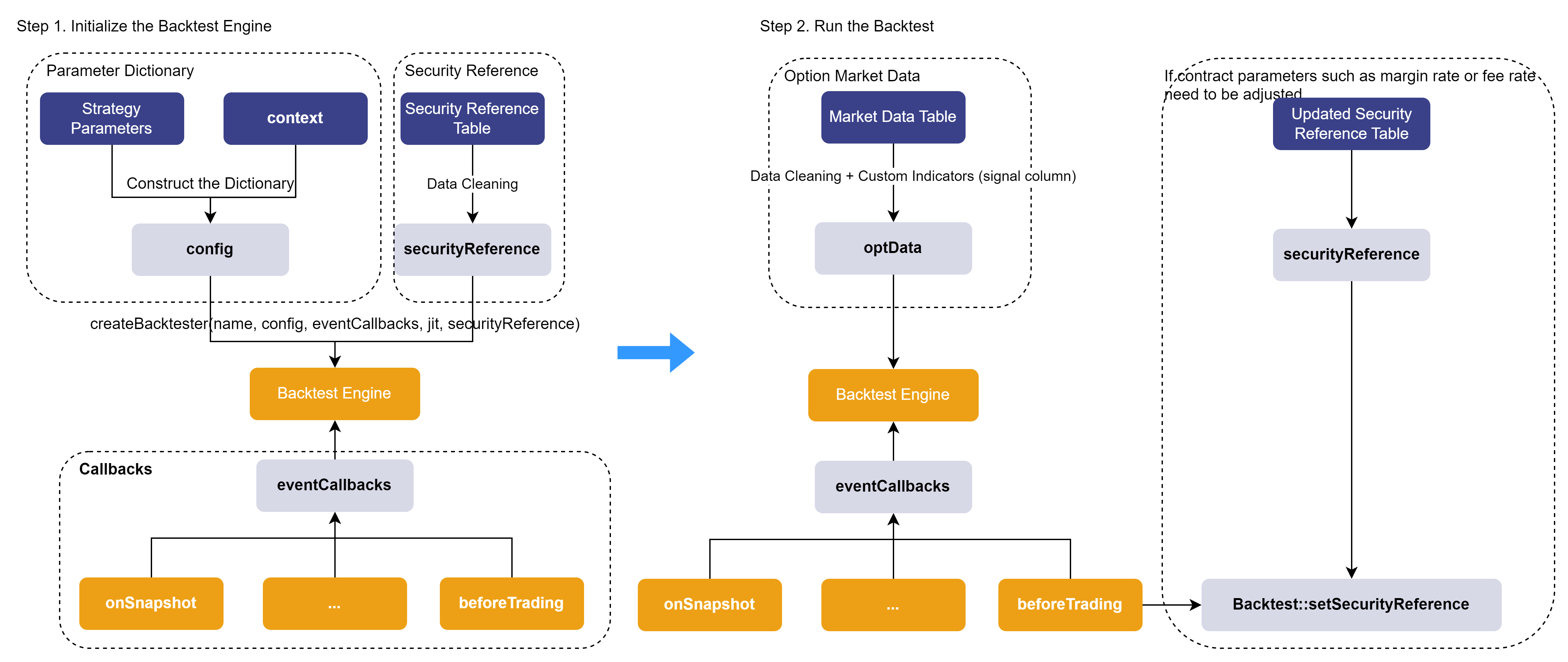
Figure 2. Figure 2-1 Workflow of Mid/High Frequency Options Backtesting

During backtesting, if parameters such as the contract’s multiplier, fee rate, or margin change, these updates can be handled in the beforeTrading pre-market callback. Then by calling Backtest::setSecurityReference with the updated reference table, the backtesting can more accurately reflect real trading conditions.

2.1 Creating the Backtesting Engine

The backtesting engine is created via the Backtest::createBacktester function, which includes the following key parameters:

eventCallbacks: a dictionary of callback functions used to define the strategy’s handling logic at different event triggers (e.g., market data updates, order matching results, etc.) (see the following paragraphs for details).
config: the engine configuration dictionary, containing various parameters required for strategy execution as well as the context dictionary for maintaining strategy state.
securityReference: the reference table of underlying contract information.

In this article, the cleaned option market data (optData) and the underlying reference table (securityReference) are saved as CSV files and provided for download in the attachments. You can load them using the loadText function.

The complete code for creating the backtesting engine is as follows:

/* 1. Create Backtesting engine */
// Option reference table
filePath = "/ssd/ssd0/single16coreJIT/server/optionData/" // Replace with the CSV path on your DolphinDB server
schemaTb = table(["symbol","underlyingAssetType","multiplier","type","strikePrice","marginRatio","tradeUnit",
                  "priceUnit","priceTick","commission","deliveryCommissionMode","lastTradingDay","exerciseDate",
                  "exerciseSettlementDate","exDate","adjStrikePrice","adjMultiplier"] as `name,
                 ["SYMBOL","INT","DOUBLE","INT","DOUBLE","DOUBLE","DOUBLE","DOUBLE","DOUBLE","DOUBLE","INT",
                 "DATE","DATE","DATE","DATE","DOUBLE","DOUBLE"] as `types)
securityReference = loadText(filePath+"optSecurityReference.csv",schema=schemaTb)
// Prepare Backtest configuration parameters
config = dict(STRING, ANY)
config["startDate"] = startDate // Backtest start date
config["endDate"] = endDate // Backtest end date
config["strategyGroup"] = "option" /// Strategy type
config["dataType"] = 1 // Use snapshot data
config["callbackForSnapshot"] = 0 // Effective when dataType==1, 0: trigger only onSnapshot, 1: trigger onSnapshot & onBar, 2: trigger only onBar
config["maintenanceMargin"] = 1.0 // Maintenance margin ratio
config["cash"] = 1000000
config["enableAlgoOrder"] = true // Enable algorithmic orders
config["outputOrderInfo"] = true // Output rejection reason
config["matchingMode"] = 3
config["latency"] = 50 // Simulated order latency (ms)
contractDict = dict(securityReference[`symbol], split(securityReference[`symbol],"-")[0])
directionDict = dict(securityReference[`symbol], securityReference[`type])
strikePriceDict = dict(securityReference[`symbol],securityReference[`strikePrice])
// Configure main contract information
mainContractDict = dict(DATE,ANY)
mainContractDict[2025.02.17] = ["AU2504"] // Store daily main contract list
// Configure context for Backtest
config["context"] = {
    // Basic information
    "lastTimeDict": dict(SYMBOL, TIMESTAMP), // {Futures symbol: last timestamp}
    "contractDict": contractDict,  // {Option symbol: Underlying futures contract}
    "directionDict": directionDict, // 1 for Call, 2 for Put
    "strikePriceDict": strikePriceDict, // {Option symbol: strike price}
    "mainContractDict": mainContractDict, // {Date: main contract list}
    // Signal settings
    "upLimit": 0.05,  // If option spread exceeds this percentage in profit direction, close both positions
    "lowLimit": 0.03,  // If option spread exceeds this percentage in loss direction, close both positions
    "longState": dict(SYMBOL, ANY), // {Futures: {Bull Call pair: [min spread, max spread]}}
    "shortState": dict(SYMBOL, ANY), // {Futures: {Bear Put pair: [min spread, max spread]}}
    // Order-related
    "lastPriceDict": dict(SYMBOL, DOUBLE), // Latest option price
    "longPair": dict(SYMBOL, ANY), // Long option pair
    "shortPair": dict(SYMBOL, ANY) // Short option pair
}
// Callback functions dictionary
eventCallBacks = dict(STRING, ANY) 
eventCallBacks["initialize"] = initialize  // Initialize function
eventCallBacks["beforeTrading"] = beforeTrading // Pre-trading callback
eventCallBacks["onSnapshot"] = onSnapshot // Snapshot callback
eventCallBacks["afterTrading"] = afterTrading // Post-trading callback
eventCallBacks["finalize"] = finalized // Finalize callback
try{Backtest::dropBacktestEngine(strategyName)}catch(ex){print(ex)}  // Remove existing Backtesting engine
// Create backtesting engine
engine = Backtest::createBacktester(strategyName, config, eventCallBacks, jit, securityReference)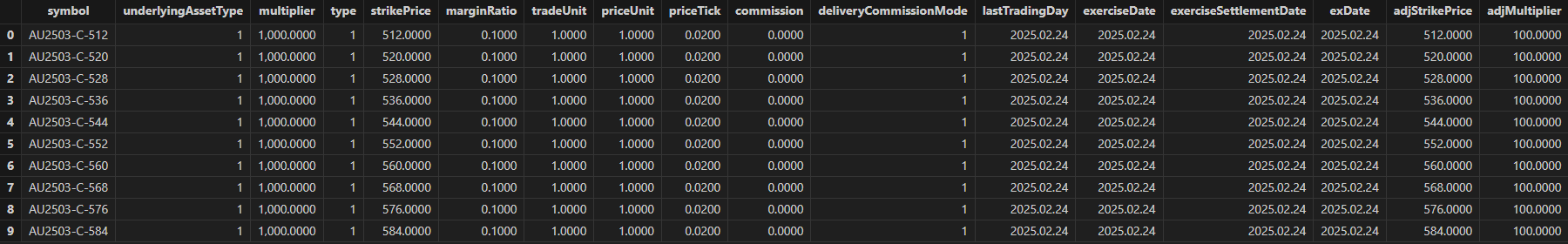

Figure 3. Figure 2-2 Option Contract Reference Data

2.2 Executing the Backtest

This section describes how to compute the three core indicators used in the strategy—option strike level, MACD trend signal, and IV signal—which are stored in the signal column. It also explains how to pass market data containing these custom indicators into the backtesting engine to execute the backtest.

Step 1. Reading Market Data

Since this strategy only involves the main contracts, only the data of the main contracts is extracted.

// Load data and execute strategy backtest
schemaTb = table(["symbol","symbolSource","timestamp","tradingDay","lastPrice",
                  "upLimitPrice","downLimitPrice","totalBidQty","totalOfferQty",
                  "bidPrice","bidQty","offerPrice","offerQty","highPrice","lowPrice",
                  "prevClosePrice","prevSettlementPrice","underlyingPrice",
                  "Theta","Vega","Gamma","Delta","IV",
                  "contract","strike","direction"] as `name, 
                  ["SYMBOL","SYMBOL","TIMESTAMP","DATE","DOUBLE","DOUBLE","DOUBLE",
                  "LONG","LONG","DOUBLE[]","LONG[]","DOUBLE[]","LONG[]","DOUBLE",
                  "DOUBLE","DOUBLE","DOUBLE","DOUBLE","DOUBLE","DOUBLE","DOUBLE",
                  "DOUBLE","DOUBLE","SYMBOL","DOUBLE","INT"] as `types)
data = select * from loadText(filePath+"optData.csv",schema=schemaTb) 
        where symbol.startsWith("AU2504") // Only trade main contract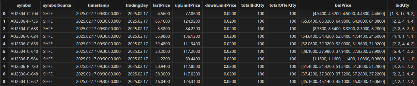

Figure 4. Figure 2-3 Snapshot Option Market Data Schema

Step 2. Computing Option Strike Levels

Once the option market data has been retrieved, the strike levels are preprocessed using vectorized SQL operations for consistent use in the subsequent strategy logic. For both calls and puts, an INT-type strike level column is output: 0 indicates ATM options, -k indicates OTM options of level k, and k indicates ITM options of level k. The SQL code for computing option strike levels is as follows:

// Compute hourly spread
hourRank = select firstNot(strike)-firstNot(underlyingPrice) as priceDiff from data 
           group by contract, tradingDay, direction, symbol, hour(timestamp) as tradeHour
// Determine level rank within each hour
update hourRank set levelRank = iif(direction == 1, 
            rank(priceDiff,true), rank(priceDiff,false)) 
            context by direction, contract, tradingDay, tradeHour 
// Find ATM option within hourly cross-section (priceDiff closest to 0)
eqData = select sum(eqRank) as eqRank from (
    select tradingDay, tradeHour, direction, contract, 
    iif(abs(priceDiff) == min(abs(priceDiff)), levelRank, 0) as eqRank from hourRank
    context by tradingDay, tradeHour, direction, contract) 
    group by tradingDay, tradeHour, direction, contract
hourData = lj(hourRank, eqData, `tradingDay`tradeHour`direction`contract)
update hourData set levelRank = eqRank-levelRank 
// Compute strikes price levels: 0=ATM, -k=OTM, +k=ITM
// Join back to original data
data = select * from data a left join (
  select contract, tradingDay, direction, symbol, tradeHour, levelRank from hourData) b
        on a.timestamp.hour() == b.tradeHour 
        and a.contract == b.contract
        and a.tradingDay == b.tradingDay 
        and a.direction == b.direction 
        and a.symbol == b.symbol
        order by timestamp asc

Step 3. Generating Opening Signals

According to the strategy, a bull call spread opening signal is triggered when MACD turns from negative to positive and IV exceeds the 30-snapshot mean plus the standard deviation; a bear put spread opening signal is triggered when MACD turns from positive to negative and IV falls below the 30-snapshot mean minus the standard deviation. The code for computing MACD and IV signals is as follows:

/* Compute MACD trend signal */
macdFunc = def (lastPrice, short_=24, long_=52, m=18) {
    dif = ewmMean(lastPrice, span=short_, adjust=false) -
    ewmMean(lastPrice, span=long_, adjust=false)
    dea = ewmMean(dif, span=m, adjust=false)
    macd = (dif - dea) * 2
    return round(macd, 4)
}
update data set macd = macdFunc(underlyingPrice).nullFill(0) context by symbol
update data set trendFactor = iif(macd>0 and prev(macd)<0, 1, 
                        iif(macd<0 and prev(macd)>0, -1, 0)) context by symbol
/* Compute IV signal */
update data set ivLongLevel = mavg(IV.ffill(), 30) - mstd(IV.ffill(), 30) context by symbol
update data set ivShortLevel = mavg(IV.ffill(), 30) + mstd(IV.ffill(), 30) context by symbol
update data set ivFactor = iif(IV<ivLongLevel, 1.0, iif(IV>ivShortLevel, -1.0, 0.0)) // IV signal

Step 4. Ingesting Data into the Engine

All custom indicators used during the backtest are merged into array vector via the fixedLengthArrayVector function and passed into the backtesting engine as part of the market data.

Finally, a data record with the symbol "END" is sent to the engine to indicate the backtest completion.

// Final data ingested into engine = market data + IV & Greeks + signals
data = select symbol, symbolSource, timestamp, tradingDay, lastPrice, upLimitPrice, downLimitPrice, 
          totalBidQty, totalOfferQty, bidPrice, bidQty, offerPrice, offerQty, highPrice, lowPrice,
          prevClosePrice, prevSettlementPrice,
          prevSettlementPrice as settlementPrice,
          underlyingPrice, Theta, Vega, Gamma, Delta, IV, 
          fixedLengthArrayVector(double(levelRank),double(ivFactor),double(trendFactor)) as signal
          from data 
          order by timestamp asc
timer Backtest::appendQuotationMsg(engine, data) // ingest snapshot data into backtesting engine
// Set END signal
endSignal = select * from data where timestamp = max(timestamp) limit 1
update endSignal set symbol = "END"
Backtest::appendQuotationMsg(engine, endSignal)
go

3. Strategy Evaluation

3.1 Strategy Results

After the overall strategy has been executed, the following functions can be used to view the backtesting results.

// View backtesting results
contextInfo = Backtest::getContextDict(engine) // Final context dictionary
tradeDetails = Backtest::getTradeDetails(engine) // Trade details table
openOrders = Backtest::getOpenOrders(engine) // Open orders at the end of day
totalPosition = Backtest::getPosition(engine)  // Current positions
dailyPosition = Backtest::getDailyPosition(engine) // Daily position table
enableCash = Backtest::getAvailableCash(engine) // Final available cash
dailyPortfolios = Backtest::getDailyTotalPortfolios(engine) // Daily P&L metrics table
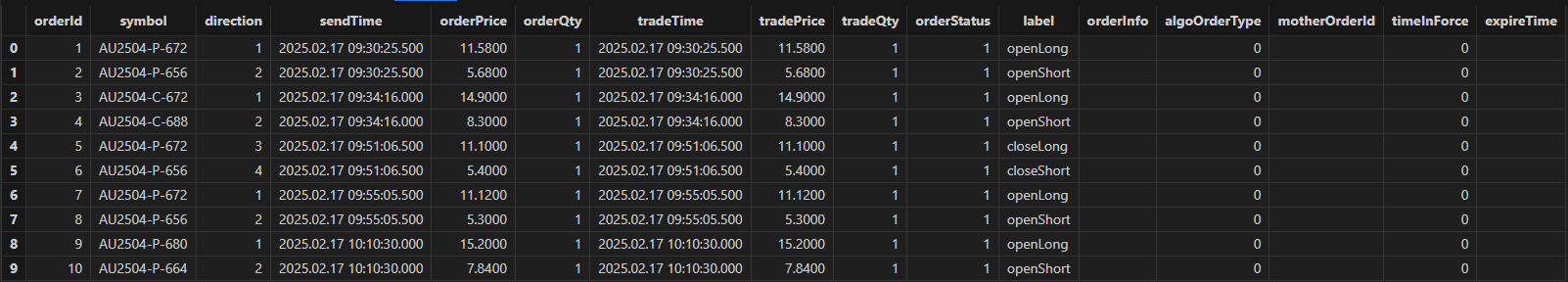
returnSummary = Backtest::getReturnSummary(engine) // Summary analytics table

Here we show the results from tradeDetails (executed orders). The figure shows that the strategy results are consistent with the trading logic:

After a bull call spread signal was triggered, at 09:30:25, the option pair AU2504-P-672 & AU2504-P-656 was executed, with a spread of 11.58 - 5.68 = 5.9.
At 09:51:06, the spread of the same option pair dropped to 11.1 - 5.4 = 5.7, reaching the lower bound of the spread change threshold, so the option pair was closed at market.

Figure 5. Figure 3-1 Strategy Trade Execution Details

3.2 Strategy Performance

The DolphinDB Backtest plugin supports JIT optimization to improve backtesting performance. When creating the backtesting engine via Backtest::createBacktester , setting the jit parameter to true enables JIT optimization. This article compares backtesting performance with and without JIT optimization using identical parameters and data. The test results are as follows:


	Ingested Records	Executed Order Count	Backtest Time	Processing Rate (records/s)
Without JIT	283,177	38	2.39 s	118,484
With JIT	283,177	38	1.51 s	187,534

Regardless of JIT, the Backtest plugin achieves a market data processing rate exceeding 100,000 records/s. Enabling JIT improves performance by over 50% compared to running without JIT.

JIT Considerations:

The DolphinDB Backtest plugin supports JIT optimization only on DolphinDB Server version 3.00.2 or above.
When enabling JIT in the Backtest plugin, in some cases the input data structure may need to be adjusted.
When JIT optimization is enabled, tables cannot be accessed directly in callback functions. To process the data, they need to be converted into dictionaries.

3.3 Test Environment Configuration

DolphinDB server was installed and configured in cluster mode. The hardware and software environments for this test are as follows:

Hardware Environment


Component	Specification
Kernel	3.10.0-1160.88.1.el7.x86_64
CPU	Intel(R) Xeon(R) Gold 5220R CPU @ 2.20GHz
Memory	512 GB

Software Environment


Component	Version / Configuration
Operating System	CentOS Linux 7 (Core)
DolphinDB Server	3.00.4 2025.09.09 LINUX_JIT x86_64
DolphinDB License Limit	16 cores, 128 GB

4. Conclusion

This article demonstrates the implementation of a snapshot-frequency option spread strategy with integrated volatility timing using the DolphinDB Backtest plugin. It also outlines the full workflow for medium- and high-frequency option strategy backtesting and provides SQL scripts for computing option strike levels and trading signals.

The core logic of the strategy is to establish directional positions at a relatively low cost using bull call spread and bear put spread option pairs based on the current underlying futures price trend and option implied volatility level, while continuously monitoring the spread of each option pair to implement profit-taking and stop-loss closures in real time.

This case highlights the Backtest plugin’s excellent performance, rich strategy trigger mechanisms, and comprehensive backtesting evaluation results, offering practical reference for medium- and high-frequency trading strategy backtesting in the FICC domain.

5. FAQ

Handling Contract Rollover in Long-Term Backtests

In long-term option backtests, the strategy needs to handle contract rollover logic. The approach differs slightly for financial and commodity options:

For financial options: the front-month contract is treated as the main contract. To track it, an in-memory table can be maintained in the context state dictionary, storing product, contract, and remaining time to expiration. The strategy determines the current main contract based on remaining days to expiration. On rollover days, both the expiring contract and the new main contract data should be ingested into the backtesting engine to allow for closing positions of the expiring contract. On non-rollover days, only the current main contract needs to be ingested.
For commodity options: the daily main contract can be identified using futures snapshot data to compute contract OHLC bars and continuous futures contracts, or by referencing an existing table of main contracts. Once identified, the corresponding contract data is ingested into the backtesting engine, with rollover handling logic following the same pattern as for financial options.

Appendix

Backtesting script: backtesting.dos
Data: data.zip